Emotional Impact on Memory Part 2
Data Prep and Analysis
This is the second part of the expriment on Pattern Separation. This processes the participants hits and misses into the induced negative or neutral group and displays some results.
Import
Raw CSV files with all IAPS database and images to be used in each task imported into an object.
raw_df <- read_csv("data/ret_task.csv"
                   , col_types = cols(CR = col_factor(levels = c("same",  "different"))
                   , Emotion = col_factor(levels = c("negative", "neutral"))
                  , Sex = col_factor(levels = c("male", "female"))))

raw_df$CorrectAnswer <- recode(raw_df$CorrectAnswer, a = "l", l = "a")
raw_df$Stimulus1.RESP <- recode(raw_df$Stimulus1.RESP, a = "l", l = "a")

# import tables

RET_SEEN <- read_csv("data/RET_SEEN.csv")
RET_UNSEEN_NEW <- read_csv("data/RET_UNSEEN_NEW.csv")
RET_PS_a <- read_csv("data/RET_PS_a.csv")
Data Setup
75 Negative Images
75 Neutral Images
General d-prime score: p(hits|75) and then p(FA|75)
| SAME(A) | DIFFERENT(L) | |
|---|---|---|
| NEW | MISS(FA) | HIT(CR) |
| OLD | MISS | MISS |
| SIMILAR | HIT | MISS |
Compute New Variables
Pattern separation scores were calculated by comparing the CorrectAnswer response to the actual Stimulus1.RESP and then allocated either a hit or miss where appropriate. Futher variables were then computed as a binary response of 1 for a hit or 0 for a miss.
Negative and Neutral conditions were also computed as when a participant responded to a hit when a image is in the negative condition. Neutral was the compliment of this.
raw_df <- raw_df %>%
  select_all() %>%
  mutate(
    Pattern_Sep = case_when(
      CorrectAnswer == Stimulus1.RESP & CorrectAnswer == "a"  ~ "Hit",
      # Condition checks to match correct answer to
      CorrectAnswer == Stimulus1.RESP & CorrectAnswer == "l" ~ "Hit",
      # the participants response. Labelled as "hits"
      CorrectAnswer != Stimulus1.RESP & CorrectAnswer == "l" ~ "Miss",
      # and "miss" for easy identifying.
      CorrectAnswer != Stimulus1.RESP & CorrectAnswer == "a" ~ "Miss",
      TRUE  ~ "")) %>%
  mutate(
    Score = case_when(
      Pattern_Sep == "Hit" ~ 1, # A column of hits and misses coded 1 for hit and 0 for miss
      Pattern_Sep == "Miss" ~ 0
    )
  )  %>%
  mutate(
    Total_Hits = factor(case_when( # total counts for hits and misses
      Score == 1 ~ 1,
      Score == 0 ~ 0
    )),
    Total_Miss = factor(case_when(
      Score == 0 ~ 1,
      Score == 1 ~ 0
    ))
  )  %>%
  mutate(Hit_similar = factor(ifelse(CorrectAnswer %in% c("a") &
                                       # These columns count the appropriate hits and misses
                                Stimulus1.RESP == "a", 1, 0)),
         # for each emotional condition.
         Negative_Hit = factor(ifelse(Emotion %in% c("negative") &
                            Pattern_Sep == "Hit", 1, 0)),
         Negative_Miss = factor(ifelse(Emotion %in% c("negative") &
                              Pattern_Sep == "Miss", 1, 0)),
         Neutral_Hit = factor(ifelse(Emotion %in% c("neutral") &
                             Pattern_Sep == "Hit", 1, 0)),
         Neutral_Miss = factor(ifelse(Emotion %in% c("neutral") &
                                 Pattern_Sep == "Miss", 1, 0)))

raw_df$Picture <-  str_remove(raw_df$Picture, ".jpg") #remove the jpg extention


# check the column picture number and compare to the originally coded
# tasks use to setup the experiment.
raw_df <- raw_df %>%
  mutate(
    coding = case_when(
      Picture %in% RET_PS_a$V1 ~ "SIMILAR",
      Picture %in% RET_UNSEEN_NEW$nr ~ "NEW",
      Picture %in% RET_SEEN$nr ~ "OLD",
      TRUE ~ ""))

# Added pattern separation counts similar to Stark(2013)
raw_df <- raw_df %>%
  mutate(pshits = ifelse(coding %in% c("SIMILAR") & Stimulus1.RESP == "a", 1, 0),
         psmiss = ifelse(coding %in% c("SIMILAR") & Stimulus1.RESP == "l", 1, 0),
         pscr = ifelse(coding %in% c("NEW") & Stimulus1.RESP == "l", 1, 0),
         psfa = ifelse(coding %in% c("NEW") & Stimulus1.RESP == "a", 1, 0))
Grouping Variables and Joining To Long Format:
Temporary tables are then created per subject based on hits and misses.
a <- raw_df %>% group_by(Subject, Neutral_Hit) %>%
  tally() %>%
  filter(Neutral_Hit == 1) %>%
  select(n) %>%
  rename(Neutral_hits = n)

b <- raw_df %>% group_by(Subject, Neutral_Miss) %>%
  tally() %>%
  filter(Neutral_Miss == 1) %>%
  select(n) %>%
  rename(Neutral_miss = n)

c <- raw_df %>% group_by(Subject, Negative_Hit) %>%
  tally() %>%
  filter(Negative_Hit == 1) %>%
  select(n) %>%
  rename(Negative_hits = n)

d <- raw_df %>% group_by(Subject, Negative_Miss) %>%
  tally() %>%
  filter(Negative_Miss == 1) %>%
  select(n) %>%
  rename(Negative_miss = n)

e <- full_join(a, b)

f <- full_join(c, d)

g <- full_join(e, f)


h <- raw_df %>%
  group_by(Subject) %>%
  filter(Total_Hits == 1) %>%
  tally() %>%
  rename("Total_hits" = n)

i <- raw_df %>%
  group_by(Subject) %>%
  filter(Total_Miss == 1) %>%
  tally() %>%
  rename("Total_miss" = n)

j <- full_join(h, i)
k <- full_join(g, j)

l <- raw_df %>%
  select(Subject, Sex, Stimulus1.RT) %>%
  group_by(Subject, Sex) %>%
  summarise(MeanRT = mean(Stimulus1.RT), )

Ret_task_a <- full_join(l, k)


m <- raw_df %>%
  select(Subject, Sex, Emotion, Stimulus1.RT) %>%
  filter(Emotion == "negative") %>%
  group_by(Subject, Sex) %>%
  summarise(Neg_RT = mean(Stimulus1.RT))

n <- raw_df %>%
  select(Subject, Sex, Emotion, Stimulus1.RT) %>%
  filter(Emotion == "neutral") %>%
  group_by(Subject, Sex) %>%
  summarise(Neut_RT = mean(Stimulus1.RT))

# ---
d1 <- raw_df %>%
  group_by(Subject) %>%
  filter(Emotion == "negative" & Hit_similar == "1") %>%
  tally() %>%
  rename("Neg_Sim_Hit" = n)

d2 <- raw_df %>%
  group_by(Subject) %>%
  filter(Emotion == "neutral" & Hit_similar == "1") %>%
  tally() %>%
  rename("Neut_Sim_Hit" = n)

Ret_task_c <- full_join(d1, d2)

# ---

Ret_task_b <- full_join(m, n)

Ret_task_d <- full_join(Ret_task_b, Ret_task_c)

Ret_task_df_temp <- full_join(Ret_task_a, Ret_task_d) # temp join of data tables

pattern_sep_scores <- raw_df %>%
  group_by(Subject, Sex) %>%
  summarise(n_hits = sum(pshits)
            , n_miss = sum(psmiss)
            , n_cr = sum(pscr)
            , n_fa = sum(psfa)) %>%
  mutate(n_hits = replace(n_hits, which(is.na(n_hits)), 0)) %>%
  mutate(n_miss = replace(n_miss, which(is.na(n_miss)), 0)) %>%
  mutate(n_cr = replace(n_cr, which(is.na(n_cr)), 0)) %>%
  mutate(n_fa = replace(n_fa, which(is.na(n_fa)), 0))


pattern_sep_scores <- pattern_sep_scores  %>%
  mutate(Perc_correct = (n_hits + n_cr)/(n_hits + n_miss + n_fa +n_cr)
         , Dprime = (n_hits/(n_hits + n_miss)-(n_fa/(n_fa + n_cr))))

Ret_task_df_join <-  full_join(Ret_task_df_temp, pattern_sep_scores)


Ret_display <- flextable(Ret_task_df_join)
Ret_display <- bold(Ret_display, part = "header")
Ret_display %>%
  autofit() %>%
  empty_blanks() %>%
  theme_zebra()
Subject | Sex | MeanRT | Neutral_hits | Neutral_miss | Negative_hits | Negative_miss | Total_hits | Total_miss | Neg_RT | Neut_RT | Neg_Sim_Hit | Neut_Sim_Hit | n_hits | n_miss | n_cr | n_fa | Perc_correct | Dprime |
1.000 | female | 0.000 | 0.000 | 0.000 | 0.000 | 0.000 | 0.000 | 0.000 | ||||||||||
2.000 | female | 1298.667 | 9 | 66 | 9 | 66 | 18 | 132 | 1436.547 | 1160.787 | 1 | 5 | 40.000 | 10.000 | 2.000 | 48.000 | 0.420 | -0.160 |
3.000 | female | 10.520 | 1 | 1 | 0.000 | 21.040 | 0.000 | 0.000 | 0.000 | 0.000 | ||||||||
4.000 | female | 1525.947 | 53 | 22 | 57 | 18 | 110 | 40 | 1542.253 | 1509.640 | 15 | 12 | 13.000 | 37.000 | 46.000 | 4.000 | 0.590 | 0.180 |
5.000 | female | 1213.780 | 63 | 12 | 63 | 12 | 126 | 24 | 1331.240 | 1096.320 | 21 | 21 | 12.000 | 38.000 | 46.000 | 4.000 | 0.580 | 0.160 |
6.000 | female | 1799.620 | 49 | 19 | 46 | 18 | 95 | 37 | 1801.160 | 1798.080 | 16 | 11 | 0.000 | 0.000 | 0.000 | 0.000 | ||
7.000 | female | 1119.413 | 69 | 6 | 69 | 6 | 138 | 12 | 1180.413 | 1058.413 | 23 | 25 | 8.000 | 42.000 | 48.000 | 2.000 | 0.560 | 0.120 |
8.000 | female | 1217.120 | 55 | 20 | 45 | 30 | 100 | 50 | 1335.933 | 1098.307 | 15 | 15 | 21.000 | 29.000 | 41.000 | 9.000 | 0.620 | 0.240 |
9.000 | female | 744.860 | 38 | 7 | 33 | 11 | 71 | 18 | 720.533 | 769.187 | 3 | 10 | 0.000 | 0.000 | 0.000 | 0.000 | ||
10.000 | female | 1304.340 | 60 | 15 | 53 | 22 | 113 | 37 | 1379.027 | 1229.653 | 15 | 13 | 9.000 | 41.000 | 44.000 | 6.000 | 0.530 | 0.060 |
11.000 | female | 1294.087 | 63 | 12 | 65 | 10 | 128 | 22 | 1435.827 | 1152.347 | 20 | 17 | 9.000 | 41.000 | 50.000 | 0.000 | 0.590 | 0.180 |
12.000 | female | 1481.853 | 57 | 17 | 62 | 13 | 119 | 30 | 1710.893 | 1252.813 | 18 | 19 | 16.000 | 34.000 | 48.000 | 2.000 | 0.640 | 0.280 |
13.000 | female | 1198.867 | 59 | 16 | 55 | 20 | 114 | 36 | 1275.653 | 1122.080 | 21 | 19 | 20.000 | 30.000 | 44.000 | 6.000 | 0.640 | 0.280 |
14.000 | female | 1226.980 | 58 | 16 | 57 | 18 | 115 | 34 | 1303.587 | 1150.373 | 14 | 14 | 10.000 | 40.000 | 0.000 | 0.000 | 0.200 | |
15.000 | male | 1439.393 | 65 | 9 | 65 | 10 | 130 | 19 | 1578.147 | 1300.640 | 22 | 19 | 6.000 | 44.000 | 45.000 | 5.000 | 0.510 | 0.020 |
16.000 | female | 1254.487 | 55 | 19 | 52 | 23 | 107 | 42 | 1300.253 | 1208.720 | 19 | 19 | 21.000 | 29.000 | 0.000 | 0.000 | 0.420 | |
17.000 | female | 1455.613 | 68 | 7 | 64 | 11 | 132 | 18 | 1567.520 | 1343.707 | 18 | 23 | 9.000 | 41.000 | 50.000 | 0.000 | 0.590 | 0.180 |
18.000 | female | 1785.653 | 56 | 19 | 55 | 20 | 111 | 39 | 1881.147 | 1690.160 | 22 | 20 | 20.000 | 30.000 | 39.000 | 11.000 | 0.590 | 0.180 |
19.000 | female | 1252.780 | 65 | 10 | 64 | 10 | 129 | 20 | 1306.613 | 1198.947 | 24 | 20 | 0.000 | 0.000 | 49.000 | 1.000 | 0.980 | |
20.000 | female | 1431.153 | 61 | 14 | 62 | 13 | 123 | 27 | 1572.253 | 1290.053 | 25 | 23 | 19.000 | 31.000 | 44.000 | 6.000 | 0.630 | 0.260 |
21.000 | male | 1131.360 | 58 | 17 | 56 | 19 | 114 | 36 | 1182.747 | 1079.973 | 16 | 15 | 12.000 | 38.000 | 45.000 | 5.000 | 0.570 | 0.140 |
22.000 | female | 1609.927 | 59 | 16 | 66 | 9 | 125 | 25 | 1662.467 | 1557.387 | 18 | 15 | 7.000 | 43.000 | 49.000 | 1.000 | 0.560 | 0.120 |
23.000 | female | 1436.047 | 67 | 8 | 68 | 6 | 135 | 14 | 1443.507 | 1428.587 | 23 | 20 | 6.000 | 44.000 | 0.000 | 0.000 | 0.120 | |
24.000 | female | 1581.807 | 67 | 8 | 58 | 16 | 125 | 24 | 1752.227 | 1411.387 | 20 | 22 | 11.000 | 39.000 | 44.000 | 6.000 | 0.550 | 0.100 |
25.000 | female | 2077.560 | 58 | 14 | 55 | 18 | 113 | 32 | 2146.667 | 2008.453 | 20 | 22 | 0.000 | 0.000 | 0.000 | 0.000 | ||
26.000 | male | 1302.447 | 62 | 13 | 52 | 23 | 114 | 36 | 1371.093 | 1233.800 | 21 | 18 | 19.000 | 31.000 | 44.000 | 6.000 | 0.630 | 0.260 |
27.000 | female | 1296.040 | 57 | 18 | 52 | 23 | 109 | 41 | 1356.547 | 1235.533 | 22 | 18 | 22.000 | 28.000 | 41.000 | 9.000 | 0.630 | 0.260 |
28.000 | male | 1613.000 | 64 | 11 | 64 | 11 | 128 | 22 | 1672.267 | 1553.733 | 19 | 18 | 6.000 | 44.000 | 47.000 | 3.000 | 0.530 | 0.060 |
29.000 | male | 1530.573 | 64 | 11 | 65 | 10 | 129 | 21 | 1603.960 | 1457.187 | 21 | 23 | 12.000 | 38.000 | 47.000 | 3.000 | 0.590 | 0.180 |
30.000 | male | 1603.767 | 62 | 11 | 67 | 7 | 129 | 18 | 1743.040 | 1464.493 | 22 | 21 | 0.000 | 0.000 | 0.000 | 0.000 | ||
31.000 | female | 1780.807 | 65 | 9 | 66 | 7 | 131 | 16 | 2002.080 | 1559.533 | 22 | 21 | 9.000 | 41.000 | 0.000 | 0.000 | 0.180 | |
32.000 | female | 1547.813 | 64 | 11 | 61 | 14 | 125 | 25 | 1741.227 | 1354.400 | 21 | 21 | 13.000 | 37.000 | 46.000 | 4.000 | 0.590 | 0.180 |
33.000 | female | 1611.207 | 54 | 21 | 56 | 19 | 110 | 40 | 1787.000 | 1435.413 | 8 | 8 | 6.000 | 44.000 | 50.000 | 0.000 | 0.560 | 0.120 |
34.000 | female | 1794.960 | 62 | 13 | 60 | 15 | 122 | 28 | 1894.760 | 1695.160 | 17 | 16 | 5.000 | 45.000 | 44.000 | 6.000 | 0.490 | -0.020 |
35.000 | female | 1505.667 | 61 | 14 | 59 | 16 | 120 | 30 | 1682.267 | 1329.067 | 17 | 20 | 14.000 | 36.000 | 47.000 | 3.000 | 0.610 | 0.220 |
36.000 | female | 1487.033 | 65 | 10 | 53 | 22 | 118 | 32 | 1606.813 | 1367.253 | 12 | 20 | 12.000 | 38.000 | 48.000 | 2.000 | 0.600 | 0.200 |
37.000 | female | 1520.327 | 68 | 7 | 66 | 9 | 134 | 16 | 1728.267 | 1312.387 | 23 | 21 | 7.000 | 43.000 | 47.000 | 3.000 | 0.540 | 0.080 |
38.000 | female | 1531.787 | 64 | 11 | 61 | 14 | 125 | 25 | 1612.973 | 1450.600 | 24 | 21 | 15.000 | 35.000 | 45.000 | 5.000 | 0.600 | 0.200 |
39.000 | female | 954.387 | 65 | 10 | 58 | 17 | 123 | 27 | 1026.227 | 882.547 | 23 | 21 | 16.000 | 34.000 | 45.000 | 5.000 | 0.610 | 0.220 |
40.000 | female | 1763.060 | 56 | 19 | 67 | 8 | 123 | 27 | 1978.973 | 1547.147 | 22 | 15 | 12.000 | 38.000 | 48.000 | 2.000 | 0.600 | 0.200 |
41.000 | male | 1261.640 | 57 | 18 | 63 | 12 | 120 | 30 | 1293.293 | 1229.987 | 17 | 14 | 10.000 | 40.000 | 49.000 | 1.000 | 0.590 | 0.180 |
42.000 | female | 1394.307 | 63 | 12 | 59 | 16 | 122 | 28 | 1407.120 | 1381.493 | 19 | 19 | 13.000 | 37.000 | 47.000 | 3.000 | 0.600 | 0.200 |
43.000 | male | 1757.800 | 65 | 8 | 59 | 10 | 124 | 18 | 1848.413 | 1667.187 | 21 | 24 | 0.000 | 0.000 | 0.000 | 0.000 | ||
44.000 | female | 1673.367 | 63 | 12 | 62 | 13 | 125 | 25 | 1843.320 | 1503.413 | 20 | 20 | 13.000 | 37.000 | 48.000 | 2.000 | 0.610 | 0.220 |
45.000 | male | 1483.727 | 58 | 17 | 64 | 11 | 122 | 28 | 1587.053 | 1380.400 | 23 | 22 | 18.000 | 32.000 | 45.000 | 5.000 | 0.630 | 0.260 |
46.000 | male | 1496.020 | 67 | 8 | 65 | 10 | 132 | 18 | 1620.120 | 1371.920 | 22 | 23 | 11.000 | 39.000 | 48.000 | 2.000 | 0.590 | 0.180 |
47.000 | female | 1354.527 | 60 | 15 | 67 | 8 | 127 | 23 | 1481.800 | 1227.253 | 24 | 17 | 11.000 | 39.000 | 47.000 | 3.000 | 0.580 | 0.160 |
48.000 | female | 1414.340 | 50 | 25 | 61 | 14 | 111 | 39 | 1449.640 | 1379.040 | 17 | 9 | 11.000 | 39.000 | 46.000 | 4.000 | 0.570 | 0.140 |
50.000 | male | 1669.833 | 58 | 17 | 62 | 13 | 120 | 30 | 1702.427 | 1637.240 | 14 | 8 | 2.000 | 48.000 | 50.000 | 0.000 | 0.520 | 0.040 |
51.000 | female | 1150.920 | 52 | 23 | 52 | 23 | 104 | 46 | 1286.360 | 1015.480 | 22 | 17 | 28.000 | 22.000 | 43.000 | 7.000 | 0.710 | 0.420 |
52.000 | male | 1635.573 | 69 | 6 | 62 | 12 | 131 | 18 | 1728.533 | 1542.613 | 18 | 22 | 0.000 | 0.000 | 50.000 | 0.000 | 1.000 | |
53.000 | female | 1553.927 | 65 | 10 | 59 | 15 | 124 | 25 | 1743.640 | 1364.213 | 21 | 20 | 11.000 | 39.000 | 0.000 | 0.000 | 0.220 | |
54.000 | female | 1379.620 | 58 | 17 | 65 | 10 | 123 | 27 | 1422.987 | 1336.253 | 23 | 15 | 13.000 | 37.000 | 48.000 | 2.000 | 0.610 | 0.220 |
55.000 | male | 2022.313 | 52 | 22 | 46 | 28 | 98 | 50 | 2056.347 | 1988.280 | 21 | 19 | 27.000 | 23.000 | 0.000 | 0.000 | 0.540 | |
56.000 | female | 1032.767 | 44 | 8 | 43 | 9 | 87 | 17 | 1141.707 | 923.827 | 11 | 10 | 0.000 | 0.000 | 0.000 | 0.000 | ||
57.000 | female | 1129.147 | 64 | 11 | 68 | 7 | 132 | 18 | 1175.320 | 1082.973 | 22 | 19 | 8.000 | 42.000 | 49.000 | 1.000 | 0.570 | 0.140 |
58.000 | female | 1311.340 | 53 | 22 | 64 | 11 | 117 | 33 | 1411.667 | 1211.013 | 20 | 11 | 12.000 | 38.000 | 48.000 | 2.000 | 0.600 | 0.200 |
59.000 | male | 1954.567 | 50 | 24 | 46 | 27 | 96 | 51 | 1985.093 | 1924.040 | 11 | 11 | 0.000 | 0.000 | 46.000 | 4.000 | 0.920 |
Validation Task Data
Validation database imported into an object
val_task <- read_csv(file = "data/val_task.csv")A table is created by grouping by each subject and then a new variable is computed for each emotion score dimension. There is also response times for each image but wont be using those for this analysis.
val_df <- val_task %>%
  group_by(Subject) %>%
  summarise(Arousal = mean(arousal.RESP), Valence = mean(valence.RESP), Dominance = mean(dominance.RESP))
Full join of both tasks to one dataframe in wide format
val_df$Subject <- as.factor(val_df$Subject)

Ret_task_df_join$Subject <- as.factor(Ret_task_df_join$Subject)

group_39_wide <- full_join(Ret_task_df_join, val_df) # Final data table with all computed results

# Display complete dataframe of the variables of interest for analysis
group_39_wide %>%
  select(Subject, Sex, Neg_Sim_Hit, Neut_Sim_Hit, Arousal, Valence, Dominance) %>%
flextable() %>%
  bold(part = "header")%>%
  autofit() %>%
  empty_blanks() %>%
  theme_zebra()
Subject | Sex | Neg_Sim_Hit | Neut_Sim_Hit | Arousal | Valence | Dominance |
1 | female | |||||
2 | female | 1 | 5 | 4.630 | ||
3 | female | |||||
4 | female | 15 | 12 | 5.360 | 3.930 | 4.170 |
5 | female | 21 | 21 | 3.980 | 3.900 | 4.970 |
6 | female | 16 | 11 | 5.100 | 4.590 | 5.630 |
7 | female | 23 | 25 | 4.670 | 4.220 | 5.590 |
8 | female | 15 | 15 | 5.410 | 4.430 | 4.930 |
9 | female | 3 | 10 | 5.210 | 4.290 | 5.190 |
10 | female | 15 | 13 | 4.300 | 5.200 | 5.520 |
11 | female | 20 | 17 | 4.180 | 4.930 | 4.860 |
12 | female | 18 | 19 | 2.210 | 4.490 | 7.840 |
13 | female | 21 | 19 | 4.520 | 4.200 | 5.290 |
14 | female | 14 | 14 | 2.760 | 6.660 | 7.580 |
15 | male | 22 | 19 | 4.270 | 3.350 | 4.980 |
16 | female | 19 | 19 | 5.580 | 4.080 | 4.310 |
17 | female | 18 | 23 | 3.880 | 4.050 | 5.770 |
18 | female | 22 | 20 | 4.290 | 5.200 | 5.590 |
19 | female | 24 | 20 | 4.230 | 4.900 | 5.790 |
20 | female | 25 | 23 | 3.920 | 5.910 | 5.530 |
21 | male | 16 | 15 | 2.360 | 5.450 | 5.350 |
22 | female | 18 | 15 | 3.940 | 4.380 | 5.270 |
23 | female | 23 | 20 | 4.680 | 3.930 | 4.580 |
24 | female | 20 | 22 | 3.660 | 4.740 | 5.830 |
25 | female | 20 | 22 | 4.980 | 4.770 | 5.080 |
26 | male | 21 | 18 | 5.290 | 3.710 | 4.400 |
27 | female | 22 | 18 | 5.070 | 4.490 | 4.860 |
28 | male | 19 | 18 | 4.360 | 4.310 | 5.090 |
29 | male | 21 | 23 | 4.980 | 4.610 | 4.920 |
30 | male | 22 | 21 | 4.050 | 4.980 | 6.200 |
31 | female | 22 | 21 | 4.260 | 4.180 | 6.890 |
32 | female | 21 | 21 | 3.660 | 4.680 | 6.230 |
33 | female | 8 | 8 | 4.870 | 3.990 | 4.890 |
34 | female | 17 | 16 | 1.730 | 3.900 | 5.090 |
35 | female | 17 | 20 | 2.510 | 4.700 | 5.110 |
36 | female | 12 | 20 | 5.180 | 3.910 | 4.870 |
37 | female | 23 | 21 | 4.700 | 5.170 | 5.040 |
38 | female | 24 | 21 | 4.010 | 5.980 | 7.030 |
39 | female | 23 | 21 | 4.270 | 4.130 | 5.760 |
40 | female | 22 | 15 | 4.460 | 4.380 | 6.570 |
41 | male | 17 | 14 | 4.990 | 3.550 | 6.760 |
42 | female | 19 | 19 | 4.640 | 4.380 | 4.970 |
43 | male | 21 | 24 | 4.050 | 4.630 | 5.200 |
44 | female | 20 | 20 | 3.120 | 4.210 | 3.290 |
45 | male | 23 | 22 | 3.850 | 4.550 | 5.620 |
46 | male | 22 | 23 | 4.180 | 4.340 | 6.520 |
47 | female | 24 | 17 | 4.990 | 4.840 | 5.270 |
48 | female | 17 | 9 | 3.780 | 5.030 | 6.120 |
50 | male | 14 | 8 | 5.250 | 4.080 | 3.850 |
51 | female | 22 | 17 | 3.420 | 4.730 | 5.150 |
52 | male | 18 | 22 | 4.430 | 4.890 | 5.840 |
53 | female | 21 | 20 | 4.790 | 4.860 | 5.450 |
54 | female | 23 | 15 | 4.820 | 4.770 | 5.670 |
55 | male | 21 | 19 | 2.630 | 6.000 | 6.780 |
56 | female | 11 | 10 | 5.700 | 3.960 | 5.260 |
57 | female | 22 | 19 | 1.090 | 5.000 | 8.760 |
58 | female | 20 | 11 | 6.780 | 3.400 | 3.990 |
59 | male | 11 | 11 | 4.480 | 3.830 | 4.940 |
Descriptives
my_fun <- function(x, num_var){
  num_var <- enquo(num_var)

  x %>%
    summarize(avg = mean(!!num_var), n = n(),
              sd = sd(!!num_var), se = sd/sqrt(n))
}

mean_response_time <- group_39_wide %>%
  group_by(Sex) %>%
  my_fun(MeanRT)

neg_similar_hits <- group_39_wide %>%
  group_by(Sex) %>%
  na.omit() %>%
  my_fun(Neg_Sim_Hit)

flextable(mean_response_time)%>%
  add_header_lines(values = c("Mean Response Times to Stimuli")) %>%
  autofit() %>%
  empty_blanks() %>%
  theme_zebra()
Mean Response Times to Stimuli | ||||
Sex | avg | n | sd | se |
male | 1564.430 | 14 | 247.320 | 66.099 |
female | 1352.464 | 44 | 389.461 | 58.713 |
flextable(neg_similar_hits) %>%
  add_header_lines(values = c("Mean Hits of Pattern Separation Scores")) %>%
  autofit() %>%
  empty_blanks() %>%
  theme_zebra()
Mean Hits of Pattern Separation Scores | ||||
Sex | avg | n | sd | se |
male | 19.444 | 9 | 3.127 | 1.042 |
female | 19.581 | 31 | 3.802 | 0.683 |
Emotion Scores
library(hrbrthemes)
# Gather variables and change to wide format
ret_long <- group_39_wide %>%
  gather(key, value, Valence, Arousal, Dominance) %>%
  select(Subject, key, value, Sex) %>%
  rename("Emotion" = key) %>%
  arrange(desc(Subject))

ggplot(data = ret_long) +
  aes(x = value) +
  geom_histogram(bins = 30, fill = "#1f78b4") +
  labs(title = "Distribution of Emotion Response Scores",
    x = "Mean Scores",
    y = "Ratings",
    subtitle = "IAPS Scores") +
  theme_ft_rc() +
  facet_wrap(vars(Emotion))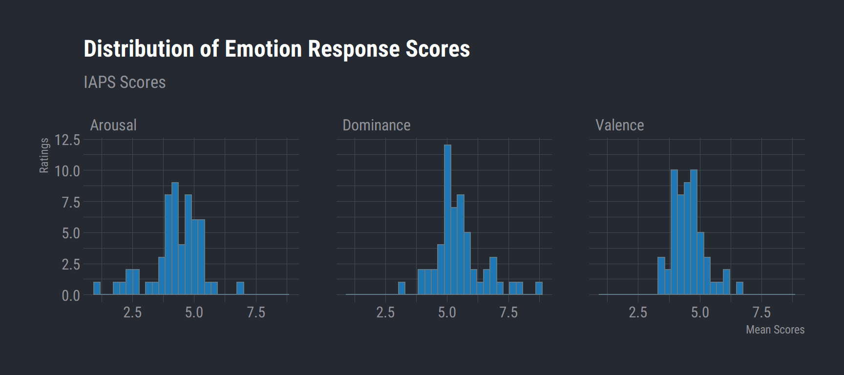
Emotion Ratings from Negative Stimuli
# Negative Emotion Scores
val_task %>%
  filter(condition == "negative") %>%
  na.omit() %>%
  group_by(Subject, Sex) %>%
  summarise(Arousal = mean(arousal.RESP)
            , Dominance = mean(dominance.RESP)
            , Valence = mean(valence.RESP)) %>%
  gather(key, value, Arousal, Dominance, Valence) %>%
  rename("Emotion" = key) %>%
  ggplot(aes(x = value)) +
  geom_histogram(bins = 20, fill = "#1f78b4") +
  labs(title = "Emotion Scores from Negative Stimuli",
       y = "Response",
    subtitle = "Arousal, Dominance and Valence") +
  theme_ft_rc() +
  facet_wrap(vars(Emotion))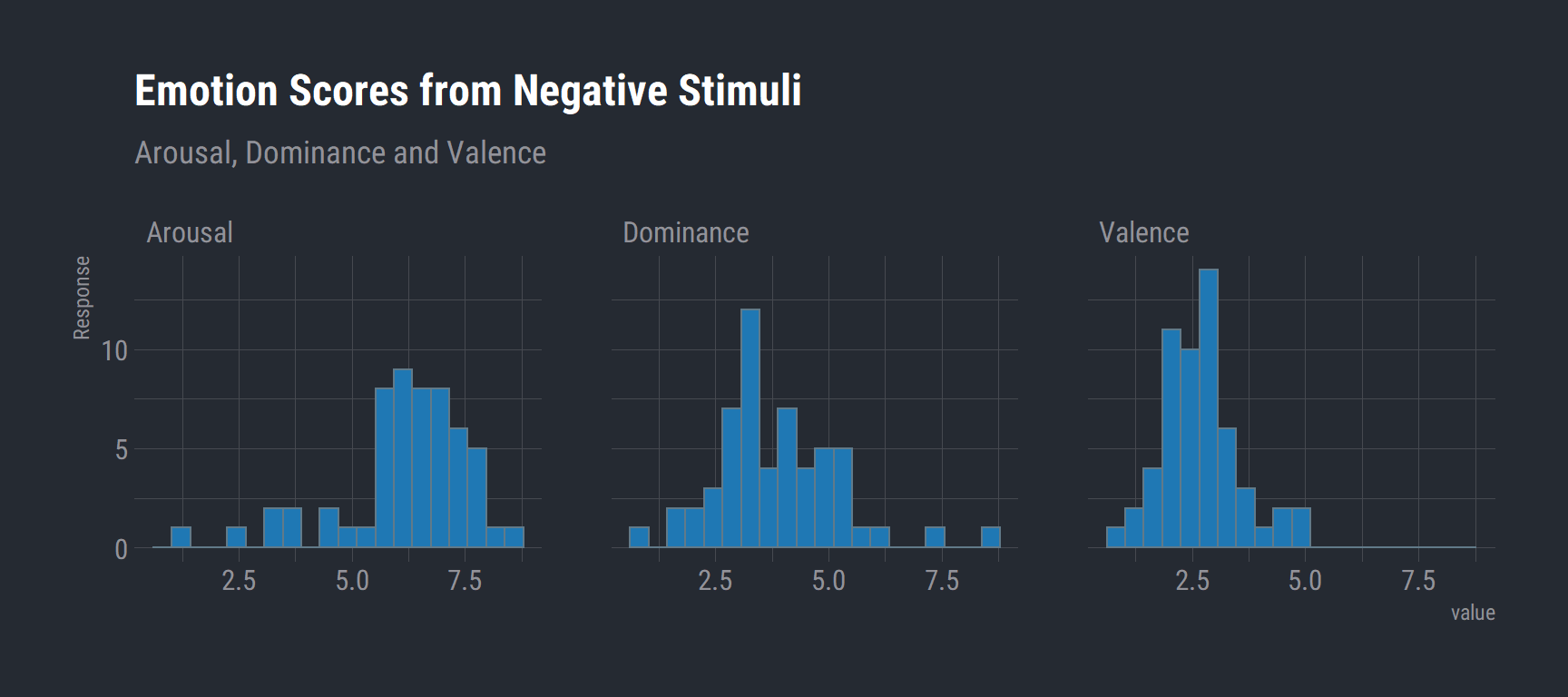
As expected, negative stimuli have a higher arousal rating and lower valence rating.
Emotion Ratings from Neutral Stimuli
# Neutral Emotion Scores
val_task %>%
  filter(condition == "neutral") %>%
  na.omit() %>%
  group_by(Subject, Sex) %>%
  summarise(Arousal = mean(arousal.RESP)
            , Dominance = mean(dominance.RESP)
            , Valence = mean(valence.RESP)) %>%
  gather(key, value, Arousal, Dominance, Valence) %>%
  rename("Emotion" = key) %>%
  ggplot(aes(x = value)) +
  geom_histogram(bins = 20, fill = "#1f78b4") +
  labs(title = "Emotion Scores from the Neutral Condition",
    subtitle = "Arousal, Dominance and Valence") +
  theme_ft_rc() +
  facet_wrap(vars(Emotion))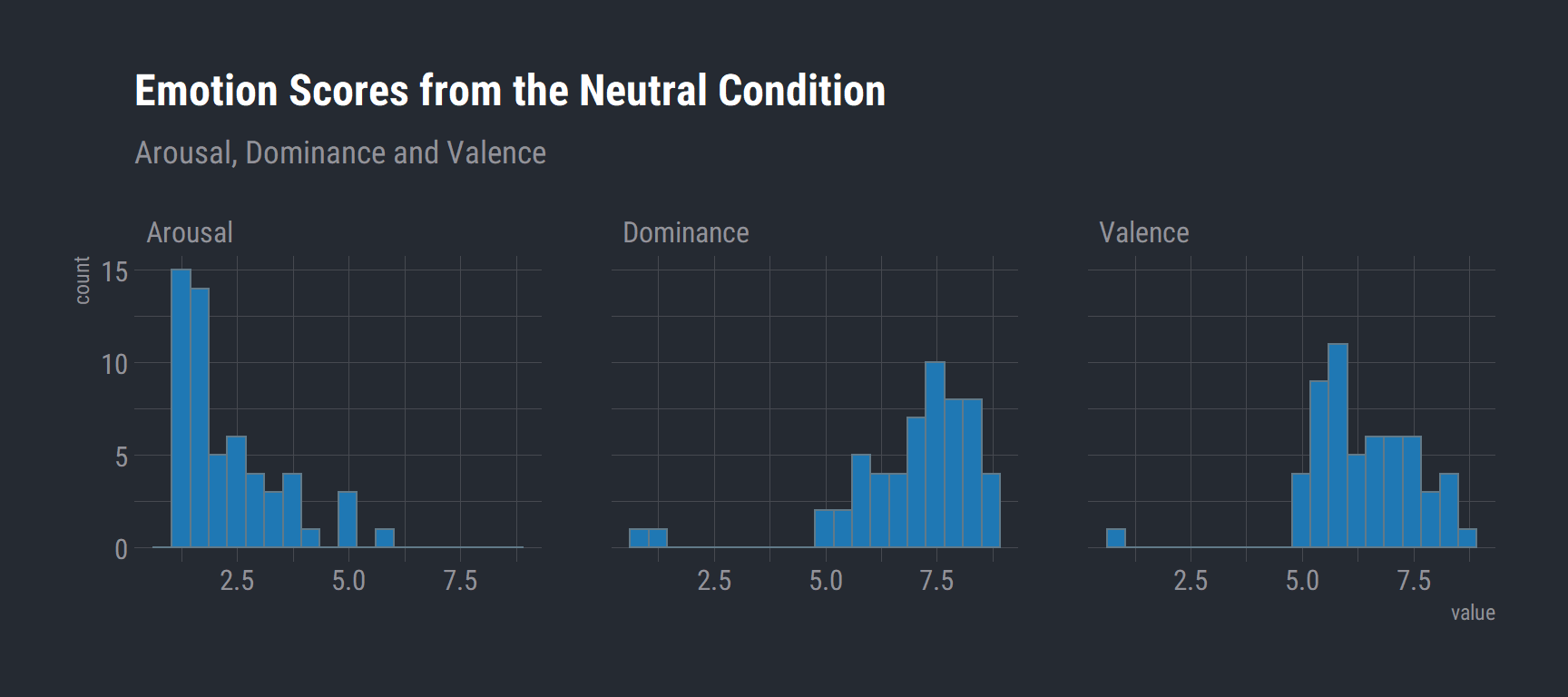
This is what we would expect. Neutral stimuli should have low arousal ratings and higher valence ratings.
Histogram of Total Negative and Neutral Condition hits
group_39_wide %>%
  gather(key, value, Neutral_hits, Negative_hits) %>% # change to long format
  select(Subject, Sex, key, value) %>%
  na.omit() %>%
  ggplot(aes(x = value)) +
  geom_histogram(bins = 22, fill = "#1f78b4") +
  theme_ft_rc() +
  facet_wrap(vars(key)) +
geom_vline(aes(xintercept = mean(value)), linetype = "dashed") 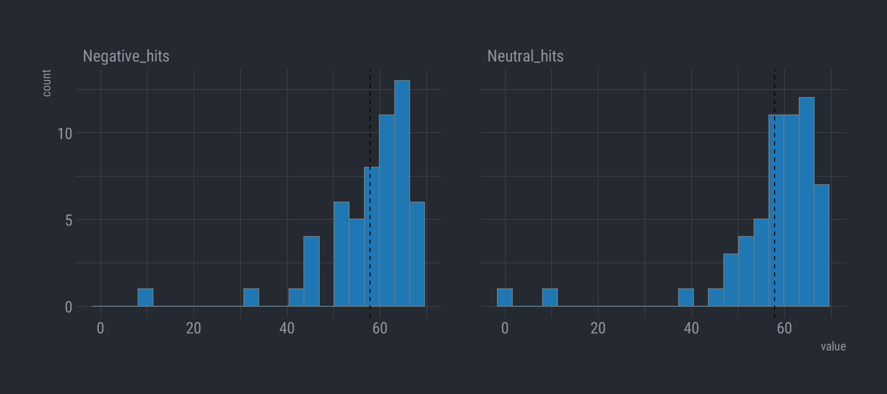
Negative Similar Hits (Male vs Females)
This is our overall indicator of if there is evidence of pattern separation performance. The ability to detect a image that was seen in the encoding task and recall if it they had seen it previously.
group_39_wide %>%
  select(Sex, Neg_Sim_Hit, Subject) %>%
  na.omit() %>%
  ggplot(aes(x = Neg_Sim_Hit)) +
  geom_histogram(bins = 22, fill = "#1f78b4") +
  labs(title = "Negative Similar Hits",
    subtitle = "Male and Females") +
  theme_ft_rc() +
  facet_wrap(vars(Sex)) +
  geom_vline(data = na.omit(group_39_wide), aes(xintercept = mean(Neg_Sim_Hit)), linetype = "dashed")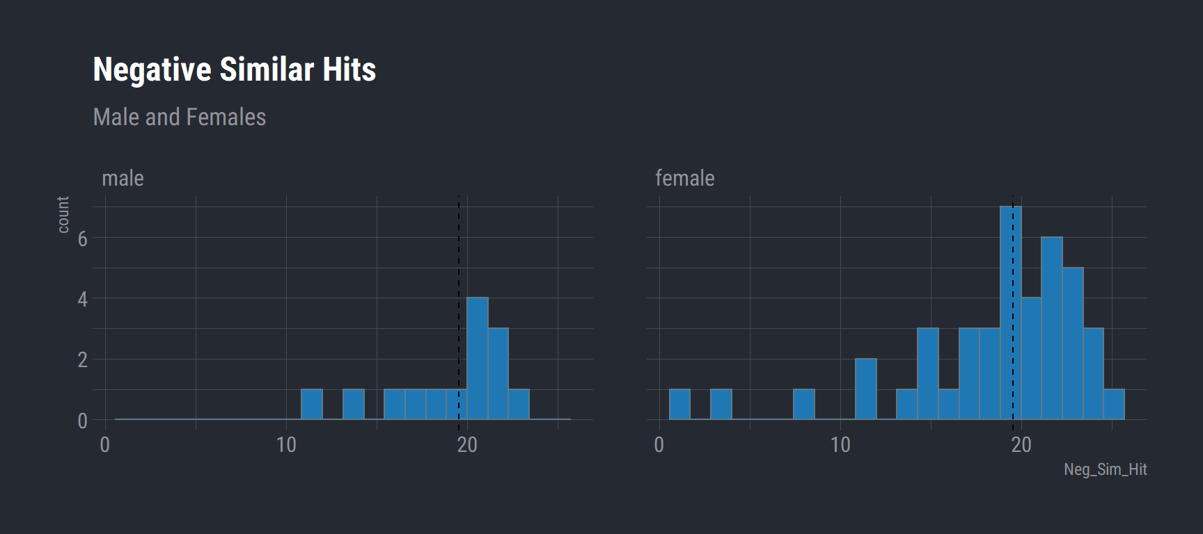
Neutral Simiar Hits (Male vs Females)
group_39_wide %>%
  select(Sex, Neut_Sim_Hit, Subject) %>%
  na.omit() %>%
  ggplot(aes(x = Neut_Sim_Hit)) +
  geom_histogram(bins = 22, fill = "#1f78b4") +
  labs(title = "Neutral Similar Hits",
       subtitle = "Male and Females") +
  theme_ft_rc() +
  facet_wrap(vars(Sex)) +
  geom_vline(data = na.omit(group_39_wide), aes(xintercept = mean(Neut_Sim_Hit)), linetype = "dashed")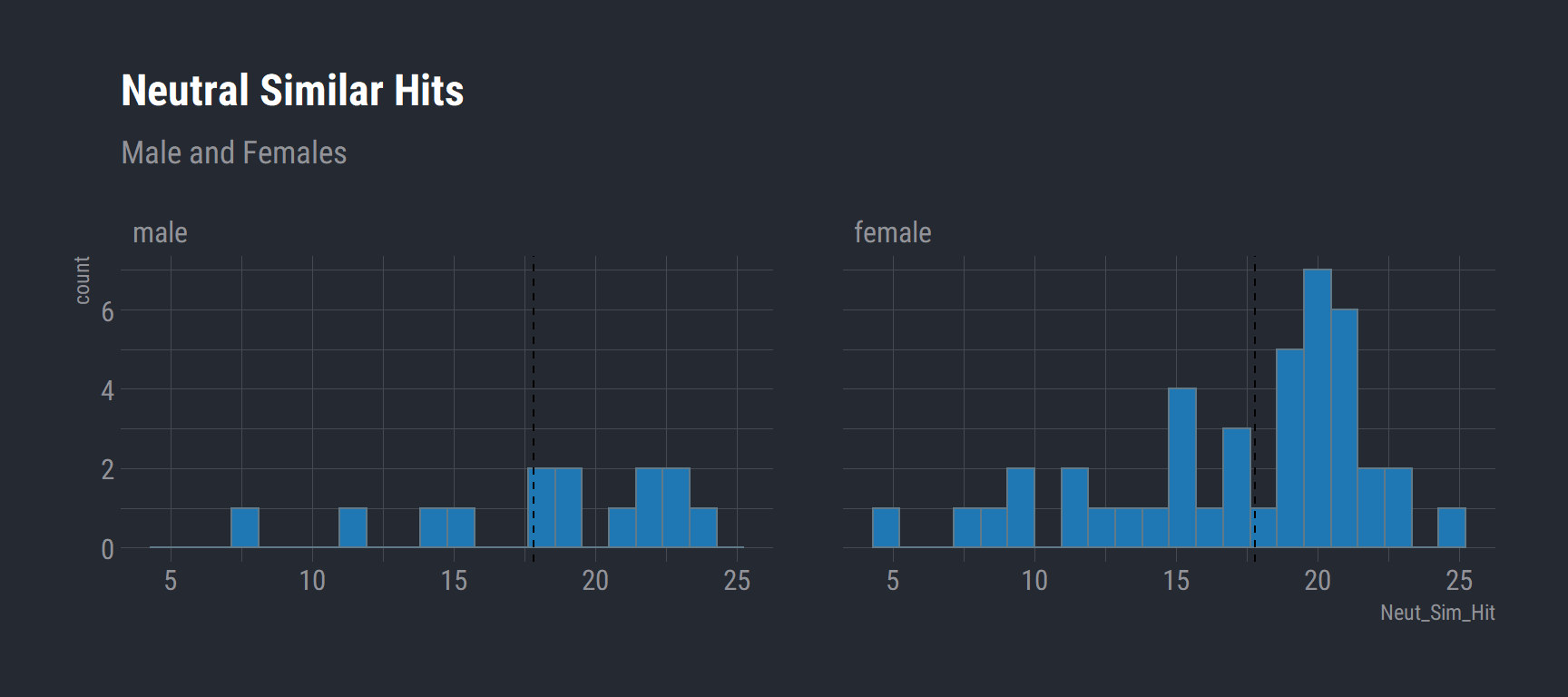
Validated vs Fake Comparisons
We need to check if the altered images were eliciting a similar emotional response as to the original IAPS validated images. There should be no difference between dimensions specifically, arousal and valence. If there is a difference then we dont know if we are actually eliciting the same response from participants as we want to.
I had already processed this file previous created a file with two groups. Group “a” is the original IAPS images with the means and sds taken from the manual. Group “b” is the altered images used in the retrieval task.
IAPS_Fake_df <- read_csv("data/validation_task_df.csv", # import data
    col_types = cols(Group = col_factor(levels = c("b",
        "a")), aromn = col_number(), dommn = col_number(),
        valmn = col_number()), na = "0")


# Change to long format

IAPS_Fake_df <- IAPS_Fake_df %>%
  gather(key, value, aromn, valmn, dommn) %>%
  rename("Emotion" = key)

IAPS_Fake_df$Emotion <- as.factor(IAPS_Fake_df$Emotion)
IAPS_Fake_df$Group <- as.factor(IAPS_Fake_df$Group)


IAPS_Fake_df %>%
  na.omit() %>%
  ggplot() +
  aes(x = Emotion, y = value, fill = Group, colour = Group) +
  geom_boxplot() +
  scale_fill_hue() +
  scale_color_hue() +
  labs(x = "Emotion"
       , y = "Mean Arousal Score"
       , title = "Validated vs Fake Comparison"
       , subtitle = "Original IAPS Images with Altered Images") +
  theme_ft_rc() +
  theme(legend.position = "none") +
  facet_wrap(vars(Group))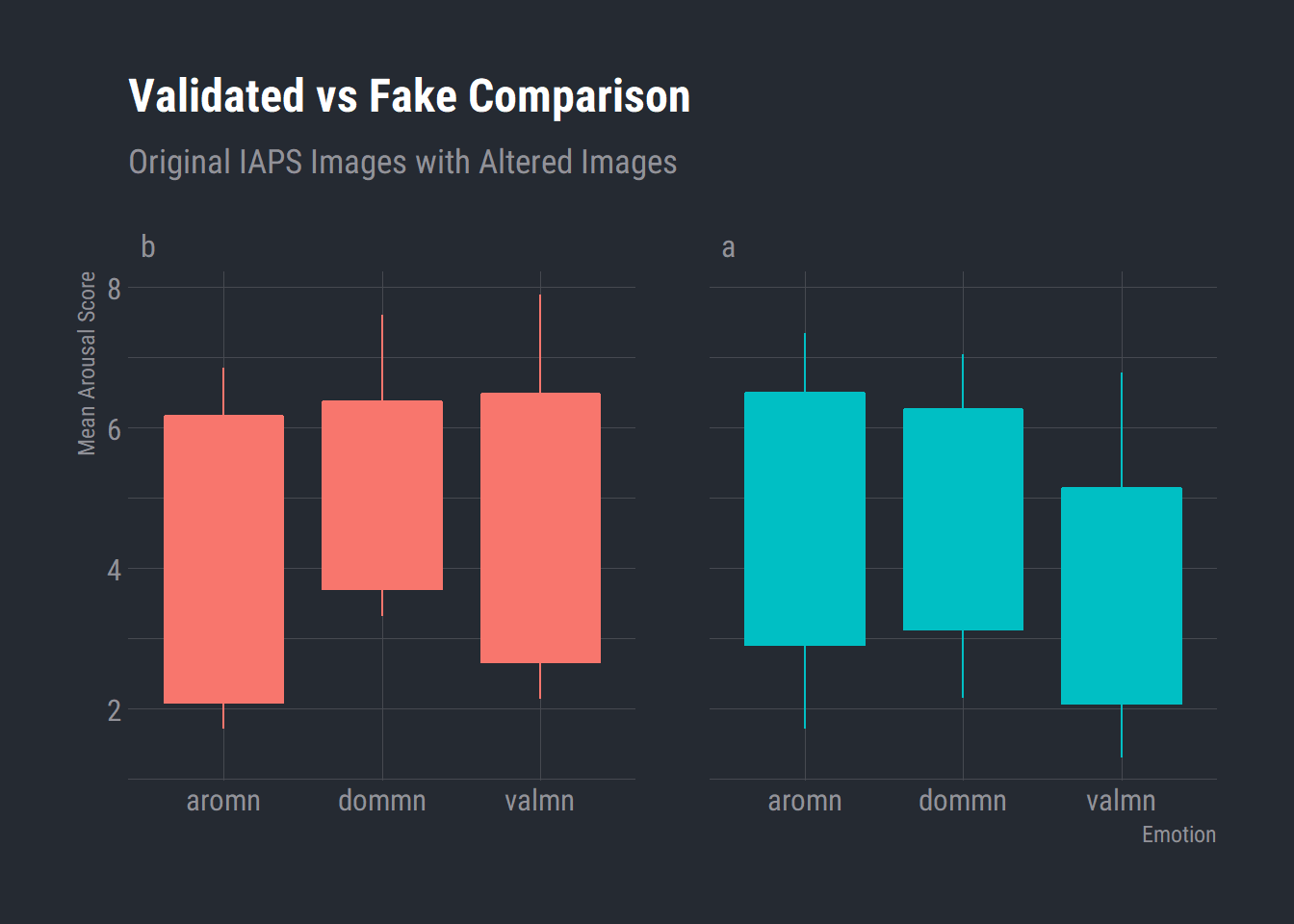
Boxplot seems to indicate we are getting pretty similar responses to the IAPS images.
library(ggpubr)

comparison <- compare_means(value ~ Emotion, group.by = "Group",  data = IAPS_Fake_df)

comparison
## # A tibble: 6 x 9
## Group .y. group1 group2 p p.adj p.format p.signif method
## <fct> <chr> <chr> <chr> <dbl> <dbl> <chr> <chr> <chr>
## 1 b value aromn dommn 0.109 0.33 0.10930 ns Wilcoxon
## 2 b value aromn valmn 0.150 0.33 0.15010 ns Wilcoxon
## 3 b value dommn valmn 0.00362 0.014 0.00362 ** Wilcoxon
## 4 a value aromn dommn 0.992 0.99 0.99175 ns Wilcoxon
## 5 a value aromn valmn 0.000505 0.0025 0.00051 *** Wilcoxon
## 6 a value dommn valmn 0.000203 0.00120 0.00020 *** WilcoxonData Analysis
Participants will show increased pattern separation scores on high arousal trials versus low-arousal trials.
We expect an interaction effect between sex and emotion, females will have a higher pattern separation score than males for negative stimuli only.
- Will need to pivot the dataframe from wide into long format
- Change the Subject and Condition variables to factors
- Run a mixed model
z <- group_39_wide %>%
  select(Subject, Sex, Neg_Sim_Hit, Neut_Sim_Hit) %>%
  gather(key = "Condition", value = "Score", Neg_Sim_Hit, Neut_Sim_Hit)

# Change to factors
z$Subject <- as.factor(z$Subject)
z$Condition <- as.factor(z$Condition)

# Run the mixed model and store in object
model <- aov(Score ~ Condition*Sex + Error(Subject/Condition), data = z)

# Summary statistics
summary(model)##
## Error: Subject
## Df Sum Sq Mean Sq F value Pr(>F)
## Sex 1 14.6 14.58 0.359 0.551
## Residuals 54 2191.7 40.59
##
## Error: Subject:Condition
## Df Sum Sq Mean Sq F value Pr(>F)
## Condition 1 41.3 41.29 6.735 0.0121 *
## Condition:Sex 1 1.7 1.71 0.280 0.5991
## Residuals 54 331.0 6.13
## ---
## Signif. codes: 0 '***' 0.001 '**' 0.01 '*' 0.05 '.' 0.1 ' ' 1# summary function does not immediately display the means for each condition, it does create a data structure that represents
# this information. And, the means can be found using model.tables
print(model.tables(model,"means"),digits=6)## Tables of means
## Grand mean
##
## 18.125
##
## Condition
## Neg_Sim_Hit Neut_Sim_Hit
## 18.7321 17.5179
## rep 56.0000 56.0000
##
## Sex
## male female
## 18.75 17.9167
## rep 28.00 84.0000
##
## Condition:Sex
## Sex
## Condition male female
## Neg_Sim_Hit 19.1429 18.5952
## rep 14.0000 42.0000
## Neut_Sim_Hit 18.3571 17.2381
## rep 14.0000 42.0000model_means <- aggregate(Score ~ Condition*Sex, data = z, mean) #Subset the means from the model
# Plot the means from the aggregated object
model_means %>%
ggplot(aes(x = Condition, y = Score, group = Sex, color = Sex, shape = Sex)) +
geom_line(size=1) +
geom_point(size=3) +
labs(x = "Emotion Condition"
, y = "Pattern Separation Score (Sim)"
, title = "Pattern Separation Scores"
, subtitle = "Males vs Females") +
theme_ft_rc()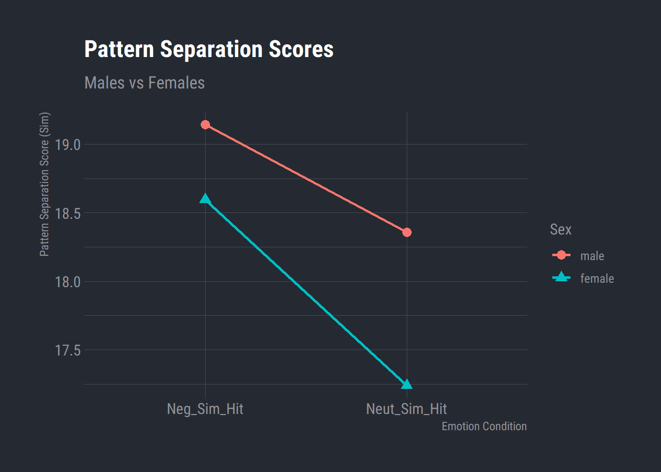
flextable(model_means)Condition | Sex | Score |
Neg_Sim_Hit | male | 19.143 |
Neut_Sim_Hit | male | 18.357 |
Neg_Sim_Hit | female | 18.595 |
Neut_Sim_Hit | female | 17.238 |
Comparison with AFEX package
As there are only 2 within conditions for each factor sphericity is assumed
library(afex)

aov_car(formula = Score ~ Condition * Sex + Error(Subject/Condition)
        , check_contrasts = afex_options("check_contrasts")
        , anova_table = list("ges")
        ,data = z) %>%
summary()##
## Univariate Type III Repeated-Measures ANOVA Assuming Sphericity
##
## Sum Sq num Df Error SS den Df F value Pr(>F)
## (Intercept) 28233.3 1 2191.7 54 695.6350 < 2e-16 ***
## Sex 14.6 1 2191.7 54 0.3593 0.55139
## Condition 24.1 1 331.0 54 3.9329 0.05245 .
## Sex:Condition 1.7 1 331.0 54 0.2797 0.59908
## ---
## Signif. codes: 0 '***' 0.001 '**' 0.01 '*' 0.05 '.' 0.1 ' ' 1group_39_wide %>%
gather(value = Score, key = Emotion, Arousal, Valence, Dominance) %>%
select(Subject, Sex, Emotion, Score) %>%
aov_car(formula = Score ~ Emotion * Sex + Error(Subject/Emotion)) %>%
summary()##
## Univariate Type III Repeated-Measures ANOVA Assuming Sphericity
##
## Sum Sq num Df Error SS den Df F value Pr(>F)
## (Intercept) 2820.11 1 24.695 53 6052.4267 < 2.2e-16 ***
## Sex 0.14 1 24.695 53 0.3005 0.5859
## Emotion 35.42 2 108.037 106 17.3748 2.975e-07 ***
## Sex:Emotion 0.05 2 108.037 106 0.0255 0.9748
## ---
## Signif. codes: 0 '***' 0.001 '**' 0.01 '*' 0.05 '.' 0.1 ' ' 1
##
##
## Mauchly Tests for Sphericity
##
## Test statistic p-value
## Emotion 0.53501 8.6586e-08
## Sex:Emotion 0.53501 8.6586e-08
##
##
## Greenhouse-Geisser and Huynh-Feldt Corrections
## for Departure from Sphericity
##
## GG eps Pr(>F[GG])
## Emotion 0.6826 1.285e-05 ***
## Sex:Emotion 0.6826 0.9312
## ---
## Signif. codes: 0 '***' 0.001 '**' 0.01 '*' 0.05 '.' 0.1 ' ' 1
##
## HF eps Pr(>F[HF])
## Emotion 0.6944999 1.114802e-05
## Sex:Emotion 0.6944999 9.337959e-01Aaron Willcox
Student
Interests include data wrangling with R and research into neurodevelopmental disorders particularly adult ADHD.