Exploring ADHD 200 Dataset

Summary Source

The ADHD-200 Sample is a grassroots initiative, dedicated to accelerating the scientific community’s understanding of the neural basis of ADHD through the implementation of open data-sharing and discovery-based science. Towards this goal, we are pleased to announce the unrestricted public release of 776 resting-state fMRI and anatomical datasets aggregated across 8 independent imaging sites, 491 of which were obtained from typically developing individuals and 285 in children and adolescents with ADHD (ages: 7-21 years old). Accompanying phenotypic information includes: diagnostic status, dimensional ADHD symptom measures, age, sex, intelligence quotient (IQ) and lifetime medication status. Preliminary quality control assessments (usable vs. questionable) based upon visual timeseries inspection are not included for all resting state fMRI scans.

In this analysis I will take a look at the distribution of scores on full IQ measures and run a regression model to look at any significant differences between typical developed children and ADHD Type.

Key

Gender

• 0 Female
• 1 Male

Handedness

• 0 Left
• 1 Right
• 2 Ambidextrous

Diagnosis

• 0 Typically Developing Children
• 1 ADHD-Combined
• 2 ADHD-Hyperactive/Impulsive
• 3 ADHD-Inattentive

ADHD Measure

• 1 ADHD Rating Scale IV (ADHD-RS)
• 2 Conners’ Parent Rating Scale-Revised, Long version (CPRS-LV)
• 3 Connors’ Rating Scale-3rd Edition

IQ Measure

• 1 Wechsler Intelligence Scale for Children, Fourth Edition (WISC-IV)
• 2 Wechsler Abbreviated Scale of Intelligence (WASI)
• 3 Wechsler Intelligence Scale for Chinese Children-Revised (WISCC-R)
• 4 Two subtest WASI
• 5 Two subtest WISC or WAIS – Block Design and Vocabulary

Medication Status

• 1 Medication Naïve
• 2 Not Medication Naïve

Quality Control

• 0 Questionable
• 1 Pass

Load Packages

library(tidyverse)
library(janitor)
library(flextable)
library(hrbrthemes)

Import Dataset and Clean

KKI <- read_csv(file = "data/nicholsn-adhd-200/KKI_phenotypic.csv") %>% 
  mutate_at(vars(`Full2 IQ`), funs(replace_na(NA))) %>% 
  select(-starts_with("QC_"))


NYU <- read_csv(file = "data/nicholsn-adhd-200/NYU_phenotypic.csv") %>% 
  mutate_at(vars(Handedness)
                  , funs(case_when(Handedness > 0.1 ~ 1,
                                   Handedness < 1 ~ 0))) %>% 
  mutate_at(vars(`Full2 IQ`), funs(replace_na(NA))) %>% 
  select(-starts_with("QC_"))
# replacing all positive-valued Edinburgh Handedness scores with a 1 
# (right-handed) and all negative scores with a 0 (left-handed)
# replace N/A with NA values

OHSU <- read_csv(file = "data/nicholsn-adhd-200/OHSU_phenotypic.csv") %>% 
  mutate_at(vars(`ADHD Index`, `Verbal IQ`, `Performance IQ`, `Full2 IQ`), funs(replace_na(NA))) %>% 
  select(-starts_with("QC_"))

Peking <- read_csv(file = "data/nicholsn-adhd-200/Peking_1_phenotypic.csv") %>% 
  mutate_at(vars(`Full2 IQ`), funs(replace_na(NA))) %>% 
  select(-starts_with("QC_"))


Pitts <- read_csv(file = "data/nicholsn-adhd-200/Pittsburgh_phenotypic.csv") %>% 
  mutate_at(vars(`ADHD Measure`, `ADHD Index`, Inattentive, `Hyper/Impulsive`), funs(replace_na(NA))) %>% 
  select(-starts_with("QC_"))


adhd_200_full_join <- bind_rows(KKI, NYU, OHSU, Peking, Pitts)


adhd_200 <- adhd_200_full_join %>% clean_names(case = "snake") %>% 
  mutate_at(vars(gender, handedness, dx, iq_measure, med_status), funs(factor)) %>% 
  mutate_all(funs(ifelse(.== -999, NA, .)))
# mutate_at with the funs changes the column in place with the function you want to run
# in this case I wanted to change them to a factor
# There were also -999 entries that need to be  replaced with NA
# If you instead want a data.frame-wise replacement of 
# a specific value (-99999) in any column for NA: mutate_all(funs(ifelse(.== -999, NA, .)))

# Generate lables for the factor levels
gender_labels <- c("Female", "Male")
adhd_200$gender <- factor(adhd_200$gender, labels = gender_labels)

hand_labels <- c("Left", "Right", "AmbiD")
adhd_200$handedness <- factor(adhd_200$handedness, labels = hand_labels)

dx_labels <- c("typical", "adhd_c", "adhd_H", "adhd_I")
adhd_200$dx <- factor(adhd_200$dx, labels = dx_labels)

x <- factor(c(NA, 2, 3, 4), exclude = NULL) 
# WISC-IV wasnt inlcuded in this dataset - only coded for 
# WASI, WISC and WASI sub type
IQ_labels <- c("WASI", "WISCCR", "WASI_sub")
adhd_200$iq_measure <- factor(adhd_200$iq_measure, labels = IQ_labels, levels = x) # This dataset only has 1 Level

x1 <- factor(c(NA, 2, 3), exclude = NULL)

md_labels <- c("Medicated", "Non_Medicated")
adhd_200$med_status <- factor(adhd_200$med_status, labels = md_labels, levels = x1)

Visualisations

inspectdf::inspect_cat(adhd_200) %>% inspectdf::show_plot(text_labels = TRUE, col_palette = 0)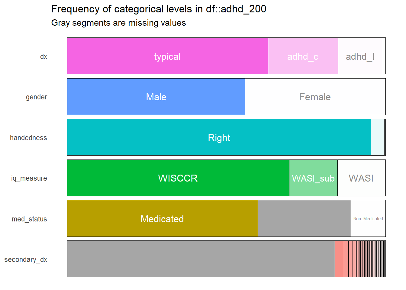

ggplot(adhd_200) +
 aes(x = age) +
 geom_histogram(bins = 30L, fill = "#0c4c8a") +
 labs(x = "Age"
      , y = "Count"
      , title = "ADHD 200 Gender Distribution"
      , subtitle = "Male and Females Aged between 8 and 13") +
 theme_ft_rc() +
 facet_wrap(vars(gender))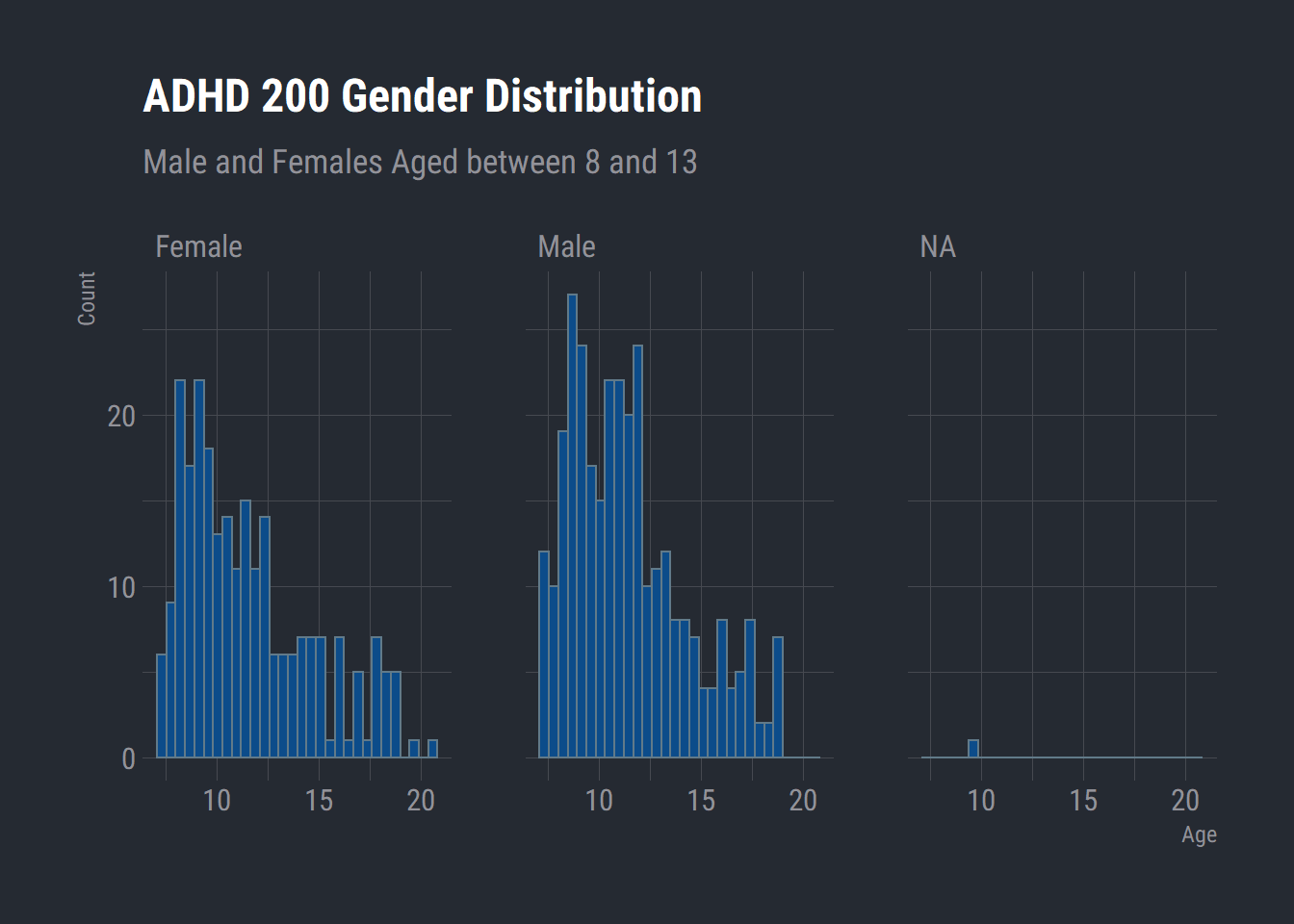

ggplot(adhd_200) +
 aes(x = full4_iq) +
 geom_histogram(bins = 30L, fill = "#0c4c8a") +
 labs(x = "Verbal IQ", title = "ADHD 200 Full IQ", subtitle = "Grouped by Type") +
 theme_ft_rc() +
 facet_wrap(vars(dx))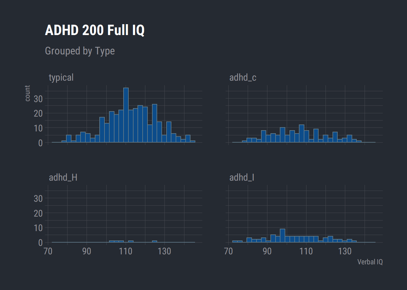

As there are non complete cases in the data frame collected from different research institutions, these can be removed for the sake of completness.

Descriptives

# Descriptives function
my_fun <- function(x, num_var){
  num_var <- enquo(num_var)
  x %>%
    summarize(Mean = mean(!!num_var, na.rm = TRUE), n = n(), 
              sd = sd(!!num_var), se = sd/sqrt(n))
}

adhd_200 %>% 
  group_by(dx, med_status) %>% 
  summarise(n = n()) %>%  
  flextable() %>% 
  autofit() %>% 
  empty_blanks() %>% 
  theme_zebra()

# Filter na cells 
adhd_200 %>% filter(!dx %in% "adhd_H") %>% 
group_by(dx, med_status) %>% 
  summarise(n = n()) %>%  
  drop_na() %>% # drop rows containing NA values
  mutate(Total = paste0(round(100 * n/sum(n), 0), "%")) %>%
   ungroup() %>%
  flextable() %>% 
  add_footer_lines(values = "NA Cells Dropped") %>% 
  set_caption("Medicated Type by ADHD Type") %>% 
  #footnote(i = 1, j = 1, value = as_paragraph(c("Footnote"))) %>% 
  autofit() %>% 
  empty_blanks() %>% 
  theme_zebra()

# ADHD Age distribution grouped by Medication Status
adhd_200 %>% group_by(dx) %>% 
  my_fun(age) %>% 
  flextable() %>% 
  bold(part = "header") %>% 
  align(align = "right", part = "all" ) %>% 
  set_header_labels(dx = "Type"
                    , Mean = "Mean Age"
                    , n = "n"
                    ,se = "se" ) %>% 
  add_header_lines(values = c("ADHD Type by Age")) %>% 
  autofit() %>% 
  empty_blanks() %>% 
  theme_zebra()

adhd_200 %>% group_by(med_status, iq_measure) %>% 
  my_fun(verbal_iq) %>% 
  drop_na() %>% # drop NA cells
  flextable() %>% 
  bold(part = "header") %>% 
  align(align = "right", part = "all" ) %>% 
  set_header_labels(med_status = "Medicated"
                    , Mean = "Mean"
                    , n = "n"
                    ,se = "se" ) %>% 
  add_header_lines(values = c("Verbal IQ by Medication")) %>% 
  autofit() %>% 
  empty_blanks() %>% 
  theme_zebra()

adhd_200 %>% group_by(med_status, iq_measure) %>% 
  my_fun(performance_iq) %>% 
  drop_na() %>% # drop NA cells
  flextable() %>% 
  bold(part = "header") %>% 
  align(align = "right", part = "all" ) %>% 
  set_header_labels(med_status = "Medicated"
                    , Mean = "Mean"
                    , n = "n"
                    ,se = "se" ) %>% 
  add_header_lines(values = c("Performance IQ by Medication")) %>% 
  autofit() %>% 
  empty_blanks() %>% 
  theme_zebra()

adhd_200 %>% group_by(med_status, iq_measure) %>% 
  my_fun(full4_iq) %>% 
  drop_na() %>% # drop NA cells
  flextable() %>% 
  bold(part = "header") %>% 
  align(align = "right", part = "all" ) %>% 
  set_header_labels(med_status = "Medicated"
                    , Mean = "Mean"
                    , n = "n"
                    ,se = "se" ) %>% 
  add_header_lines(values = c("Full IQ by Medication")) %>% 
  autofit() %>% 
  empty_blanks() %>% 
  theme_zebra()

adhd_200 %>% 
  group_by(gender) %>% 
  count() %>% 
  flextable() %>% 
  bold(part = "header") %>% 
  align(align = "right", part = "all" ) %>% 
  add_header_lines(values = c("Gender Frequency")) %>% 
  autofit() %>% 
  empty_blanks() %>% 
  theme_zebra()

Group differences

Will have a look at the group differences between ADHD Type and typically developed children on IQ measures to check for any signifcant differences.

adhd_200 %>% group_by(dx) %>%  count() %>%  flextable()

model <- adhd_200 %>% 
  select(gender, dx, med_status, age, performance_iq, verbal_iq, full4_iq) %>% 
  filter(!dx %in% "adhd_H") %>% 
  group_by(dx) %>% 
  lm(full4_iq ~ dx + gender + med_status + age, performance_iq, verbal_iq, data =.)

summary(model)

## 
## Call:
## lm(formula = full4_iq ~ dx + gender + med_status + age, data = ., 
##     subset = performance_iq, weights = verbal_iq)
## 
## Weighted Residuals:
##      Min       1Q   Median       3Q      Max 
## -182.320 -104.627   -8.884   78.792  248.145 
## 
## Coefficients:
##                         Estimate Std. Error t value Pr(>|t|)    
## (Intercept)             108.1360     4.4261  24.432  < 2e-16 ***
## dxadhd_c                -10.7634     2.2306  -4.825 2.50e-06 ***
## dxadhd_I                 -1.1875     3.0935  -0.384  0.70141    
## genderMale                9.7335     1.7328   5.617 5.42e-08 ***
## med_statusNon_Medicated  -6.3558     2.1169  -3.002  0.00297 ** 
## age                       0.1395     0.4358   0.320  0.74920    
## ---
## Signif. codes:  0 '***' 0.001 '**' 0.01 '*' 0.05 '.' 0.1 ' ' 1
## 
## Residual standard error: 125.9 on 237 degrees of freedom
##   (310 observations deleted due to missingness)
## Multiple R-squared:  0.2328, Adjusted R-squared:  0.2166 
## F-statistic: 14.38 on 5 and 237 DF,  p-value: 2.663e-12

# Means on Full IQ measurements between ADHD type and whether they are medicated or non-medicated
MM_mm <- emmeans::emmeans(model, "dx", by = "med_status")

pairs(MM_mm, type = "response")

## med_status = Medicated:
##  contrast         estimate   SE  df t.ratio p.value
##  typical - adhd_c    10.76 2.23 237  4.825  <.0001 
##  typical - adhd_I     1.19 3.09 237  0.384  0.9220 
##  adhd_c - adhd_I     -9.58 3.24 237 -2.957  0.0096 
## 
## med_status = Non_Medicated:
##  contrast         estimate   SE  df t.ratio p.value
##  typical - adhd_c    10.76 2.23 237  4.825  <.0001 
##  typical - adhd_I     1.19 3.09 237  0.384  0.9220 
##  adhd_c - adhd_I     -9.58 3.24 237 -2.957  0.0096 
## 
## Results are averaged over the levels of: gender 
## P value adjustment: tukey method for comparing a family of 3 estimates

plot(MM_mm, comparisons = TRUE)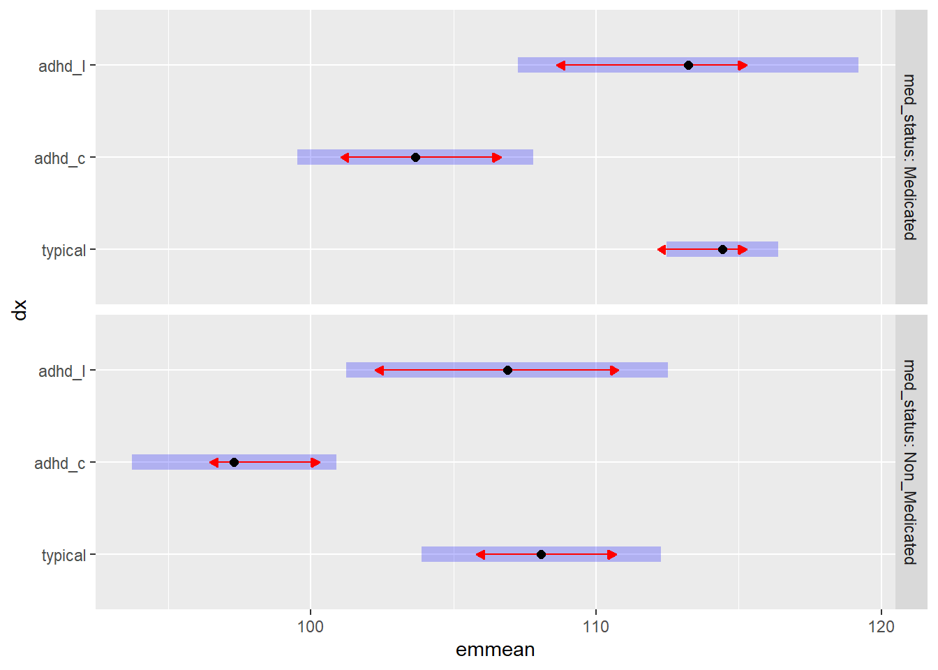

The blue bars are confidence intervals for the EMMs, and the red arrows are for the comparisons among them. If an arrow from one mean overlaps an arrow from another group, the difference is not “significant,” based on the adjust setting (which defaults to “tukey”) and the value of alpha (which defaults to 0.05)