Global Suicides 1995 to 2015
R Markdown
Import dataset
suicide_raw <- read_csv("data/master.csv")
suicide_df <- suicide_raw %>%
  select(country
         , year
         , "No_of_Suicides" =`suicides_no`
         , "ave_suicide_100k" = `suicides/100k pop`
         , sex
         , age
         , population
         , "HDI" = `HDI for year`
         , "GDP_per_year" = `gdp_for_year ($)`
         , "GDP_per_capita" = `gdp_per_capita ($)`
         , generation)

# converts to factors
suicide_df$sex <- factor(suicide_df$sex, levels = c("male", "female"))
suicide_df$year <- factor(suicide_df$year)
suicide_df$generation <- factor(suicide_df$generation)
suicide_df$country <- factor(suicide_df$country)

suicide_df$generation <- factor(suicide_df$generation,
                   ordered = T,
                   levels = c("G.I. Generation",
                              "Silent",
                              "Boomers",
                              "Generation X",
                              "Millenials",
                              "Generation Z"))
Explore dataset
Take a look at the top 50 global number of suicides from 1985 to 2015 and split by sex.
Total Amount of Suicides from 1995 to 2015
suicide_df %>%
  group_by(country, sex) %>%
  summarise(Suicide_total = sum(No_of_Suicides)) %>%
  arrange(desc(Suicide_total))  %>%
  head(50) %>%
  ggplot(aes(x = reorder(country, -Suicide_total), y = Suicide_total)
  ) +
  geom_col(show.legend = FALSE, alpha = 0.7) +
  coord_flip() +
  facet_wrap(~sex) +
labs(x = "Country", y = "Suicides 1995 to 2015", title = "Total Number of Suicides from 1985 to 2015") 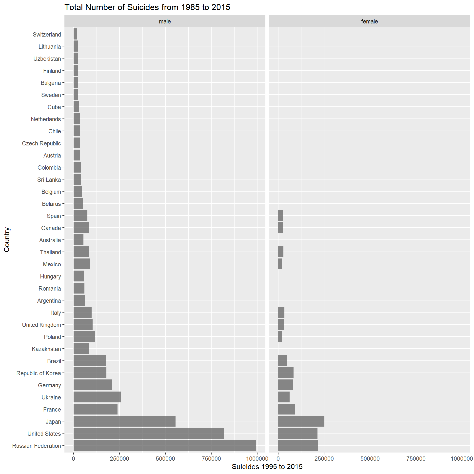
The Russian Federation has had the most amount of people commit suicide between 1985 to 2015. Following this, United States and Japan have a high number of suicides with Males commiting suicide more than Females.
Average suicide rate per population of 100,000
ave_suicide_100k_country <- suicide_df %>%
  group_by(country) %>%
  summarise(n = n(), Ave = mean(ave_suicide_100k)) %>%
  arrange(desc(Ave))


ave_suicide_100k_year <- suicide_df %>%
  group_by(country, year) %>%
  summarise(n = n(), Ave = mean(ave_suicide_100k)) %>%
  arrange(desc(Ave))


# reorder the country
ave_suicide_100k_country$country <- factor(ave_suicide_100k_country$country,
                          ordered = T,
                          levels = rev(ave_suicide_100k_country$country))

average_suicide_no <- (mean(ave_suicide_100k_country$Ave))

ave_suicide_100k_country %>%
  ggplot(aes(x = country, y = Ave)) +
  geom_bar(stat = "identity") +
  geom_hline(yintercept = average_suicide_no, linetype = 2, color = "grey35", size = 1) +
  labs(title = "Global suicides per 100k, by Country",
       caption = "1985 to 2015",
       x = "Country",
       y = "Suicides per 100k") +
  coord_flip() +
scale_y_continuous(breaks = seq(0, 45, 2)) 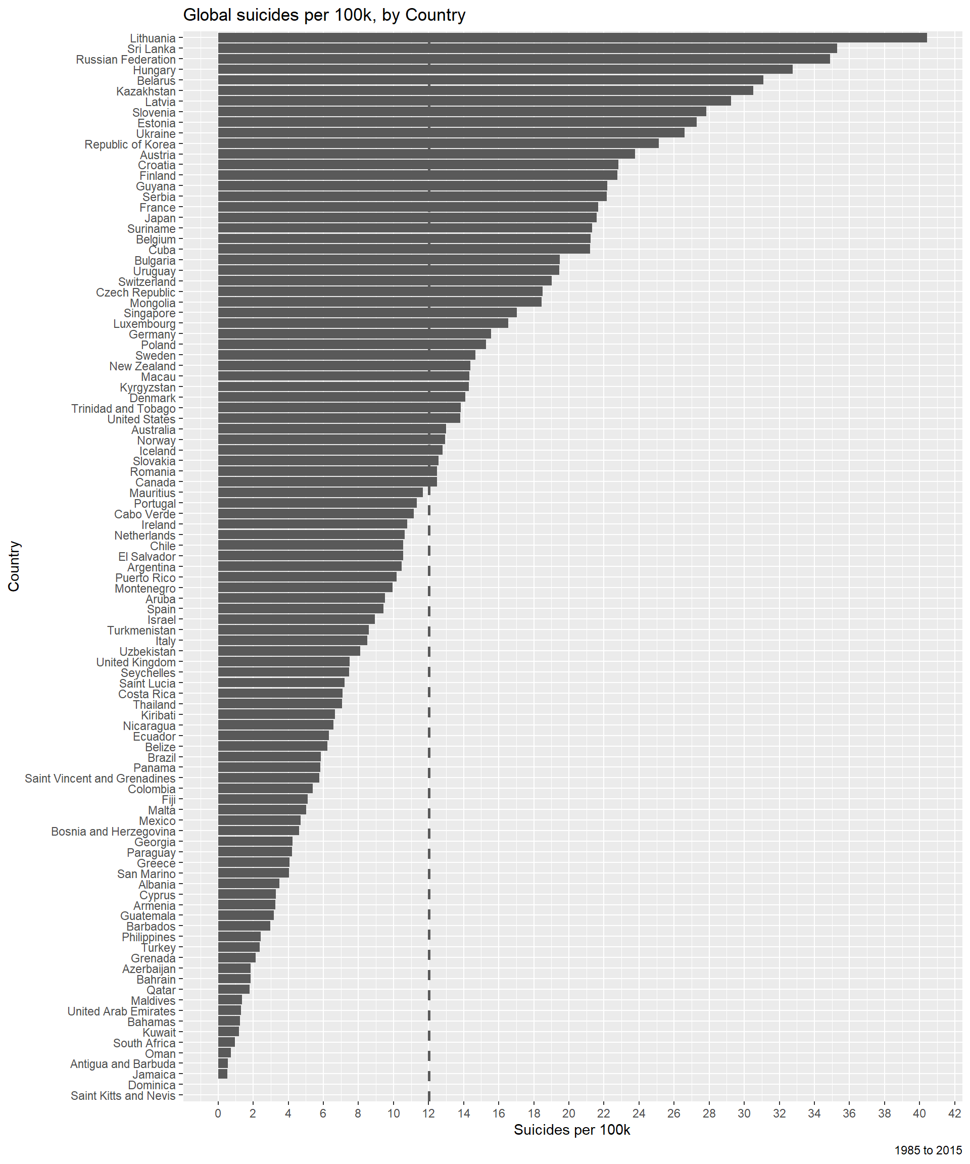
Total Average Suicide Rate per Generation between 1985 to 2015
- Gen Z, iGen, or Centennials: Born 1996 – TBD
- Millennials or Gen Y: Born 1977 – 1995
- Generation X: Born 1965 – 1976: 15 - 24 years
- Baby Boomers: Born 1946 – 1964
- Traditionalists or Silent Generation: Born 1945 and before
ave_suicide_100k_gen <- suicide_df %>%
  group_by(generation) %>%
  summarise(n = n(), Ave = sum(No_of_Suicides)) %>%
  arrange(desc(Ave))

ave_suicide_100k_gen$generation <- factor(ave_suicide_100k_gen$generation,
                          ordered = T,
                          levels = rev(ave_suicide_100k_gen$generation))

ggplot(data = ave_suicide_100k_gen) +
  aes(x = generation, weight = Ave) +
  geom_bar(fill = "#0c4c8a") +
  labs(title = "Total Suicides per Generation",
    x = "Generation",
    y = "Average Suicide Rate",
    subtitle = "1985 to 2015") +
  theme_bw() +
  coord_flip()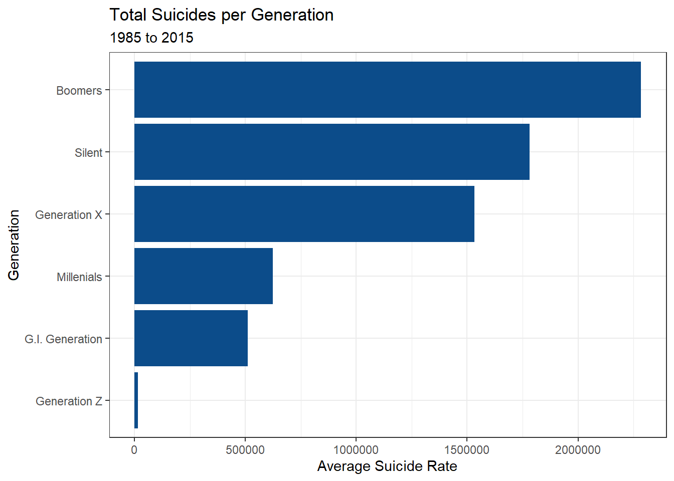
Total Amount of Suicides per country by Age (1985 to 2015)
x <- suicide_df %>%
  group_by(country, age) %>%
  summarise(total = sum(No_of_Suicides)) %>%
  filter(total > 2000) %>%
  arrange(desc(total))

ggplot(x, aes(x = reorder(country, - total), y = total, fill = age)) +
  geom_bar(stat = "identity") +
  labs(title = "Total Amount of Suicides per country by Age (1985 to 2015)",
       subtitle = "Filtered by Suicides greater than 2000",
       x = "Country",
       y = "Total Amount of Suicides",
       fill = "age") +
  coord_flip() +
  theme(legend.position = "bottom")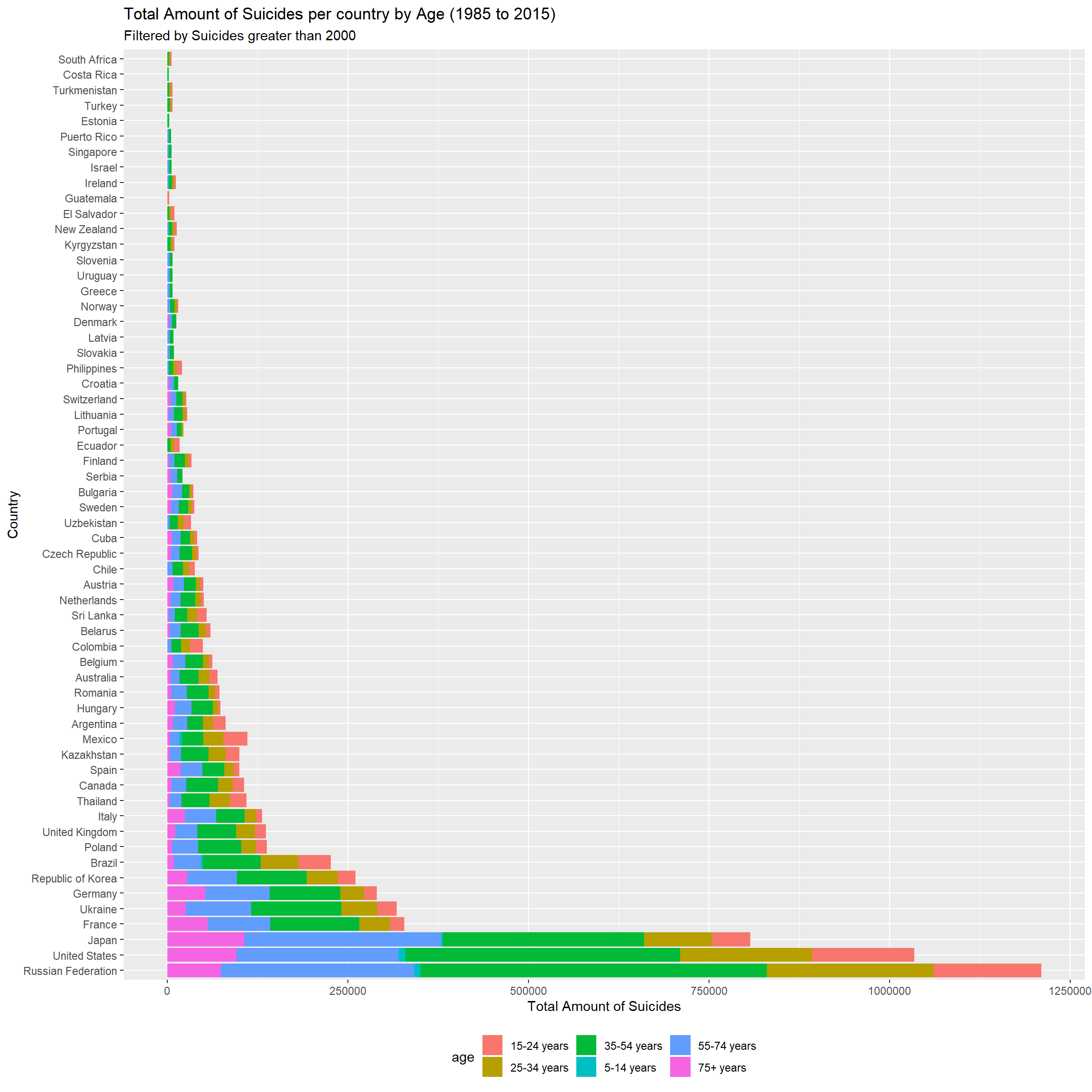
Age group of 15 to 24 years has been a consistant marker for suicides. To Explore this further, we can look at a scatter plot ages over time. Will also remove the 5 to 14 years age group.
# line graph by age group


all_age_group <- suicide_df %>%
  group_by(year, age) %>%
 filter(!(age %in% "5-14 years")) %>%
  filter(!(year %in% "2016")) %>%
  #na.omit() %>%
  summarise(Num = sum(No_of_Suicides))

ggplot(all_age_group) +
 aes(x = year, y = Num, fill = age, colour = age, group = age) +
 geom_point(size = 2.2) +
  geom_line() +
 labs(x = "Year", y = "Total Num Suicides", title = "Total Suicides per Age Group") +
 theme_bw()+
  theme(axis.text.x = element_text(angle = 90, hjust = 1))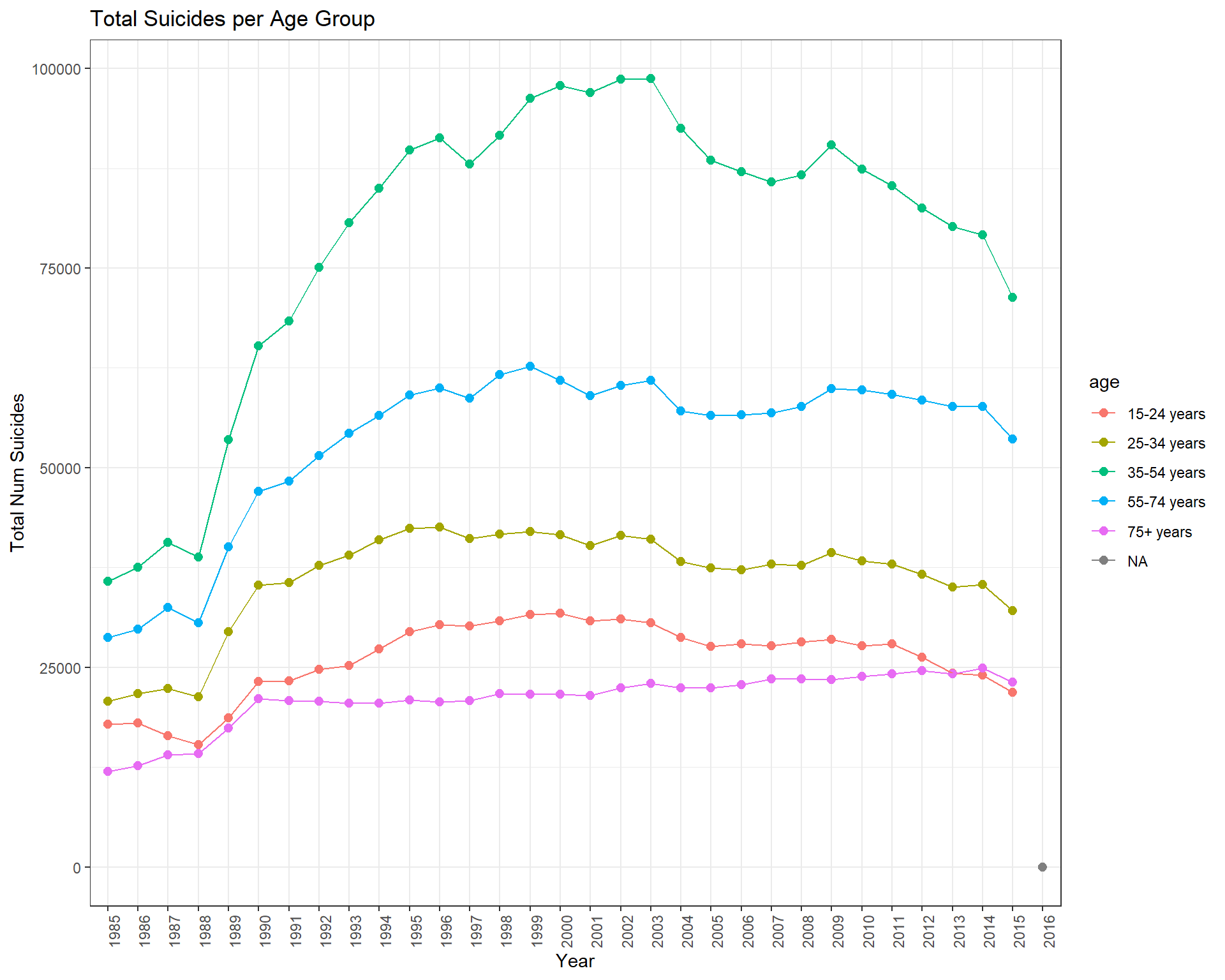
Regression model
We can use a regression model to see which age group is most likely to attempt suicide.
model <- suicide_df %>%
  lm(No_of_Suicides ~ GDP_per_year + age + sex + generation, data = .)

model %>%
  tidy(conf.int = TRUE) %>%
  filter(term != "(Intercept)") %>%
  mutate(term = fct_reorder(term, estimate)) %>% # almost always remove this
  ggplot(aes(estimate, term)) +
  geom_point() +
  geom_errorbarh(aes(xmin = conf.low, xmax = conf.high))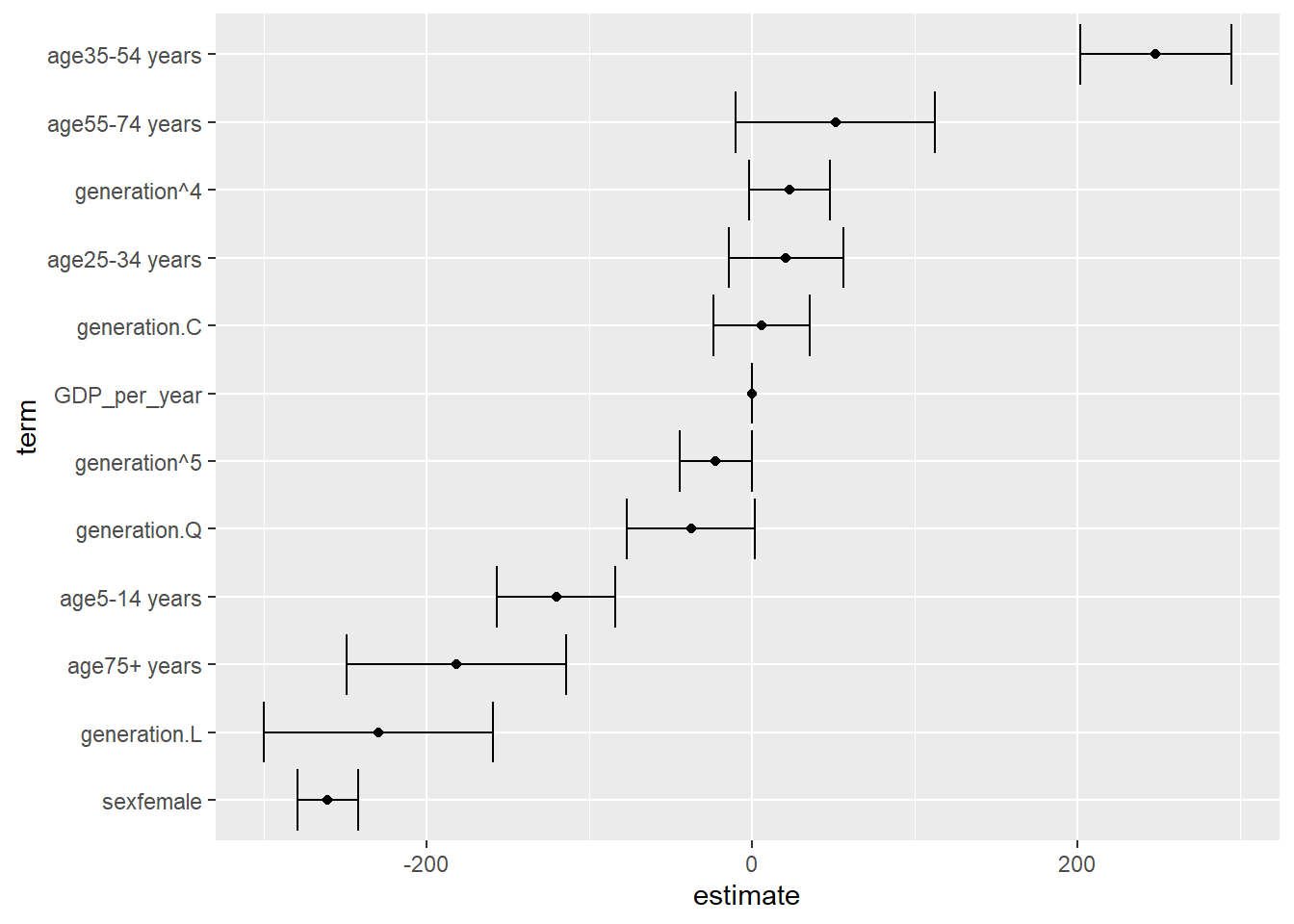
# model %>%
#  augment(data = suicide_df) %>%
#  ggplot(aes(.fitted, No_of_Suicides)) +
#  geom_point(alpha = .1)

tidy(anova(model)) %>%
mutate(Unique = sumsq / sum(sumsq))## # A tibble: 5 x 7
## term df sumsq meansq statistic p.value Unique
## <chr> <int> <dbl> <dbl> <dbl> <dbl> <dbl>
## 1 GDP_per_year 1 4187272638. 4187272638. 6777. 0. 0.185
## 2 age 5 757335476. 151467095. 245. 3.76e-257 0.0335
## 3 sex 1 473491889. 473491889. 766. 2.07e-166 0.0209
## 4 generation 5 36328382. 7265676. 11.8 2.22e- 11 0.00160
## 5 Residuals 27807 17181626084. 617889. NA NA 0.759A rough look at the effects supports previous assumptions that being male and aged between 35 - 54 years are at a higher risk of suicide. Although there might well be some collinearity between generation and age groups as these are essentially capturing similar items. I will also remove the 5 -14 year old age group as this doesnt seem to be adding anything to the model.
model2 <- suicide_df %>%
  filter(!(age %in% "5-14 years")) %>%
  lm(No_of_Suicides ~ GDP_per_year + age + sex, data = .)

model2 %>%
  tidy(conf.int = TRUE) %>%
  filter(term != "(Intercept)") %>%
  mutate(term = fct_reorder(term, estimate)) %>% # almost always remove this
  ggplot(aes(estimate, term)) +
  geom_point() +
  geom_errorbarh(aes(xmin = conf.low, xmax = conf.high))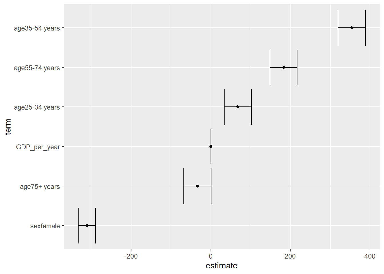
tidy(anova(model2)) %>%
  mutate(Unique = sumsq / sum(sumsq))
## # A tibble: 4 x 7
## term df sumsq meansq statistic p.value Unique
## <chr> <int> <dbl> <dbl> <dbl> <dbl> <dbl>
## 1 GDP_per_year 1 4959288738. 4959288738. 7036. 0. 0.222
## 2 age 4 460837808. 115209452. 163. 3.10e-138 0.0206
## 3 sex 1 561837996. 561837996. 797. 1.87e-172 0.0252
## 4 Residuals 23203 16354227025. 704832. NA NA 0.732Interestly, men aged between 35 - 54 years old have the strongest effect on the number of suicides followed by the 55 to 74 year old age group then young adults.
Take a look at Suicide Rate in Australia
au_model <- suicide_df %>%
  filter(country %in% "Australia") %>%
  group_by(year, sex, age) %>%
  summarise(No_of_Suicides = sum(No_of_Suicides), GDP_per_year = mean(GDP_per_year))

model2 <- au_model %>%
  filter(!(age %in% "5-14 years")) %>%
  lm(No_of_Suicides ~ GDP_per_year + age + sex, data = .)

model2 %>%
  tidy(conf.int = TRUE) %>%
  filter(term != "(Intercept)") %>%
  mutate(term = fct_reorder(term, estimate)) %>% # almost always remove this
  ggplot(aes(estimate, term)) +
  geom_point() +
  geom_errorbarh(aes(xmin = conf.low, xmax = conf.high))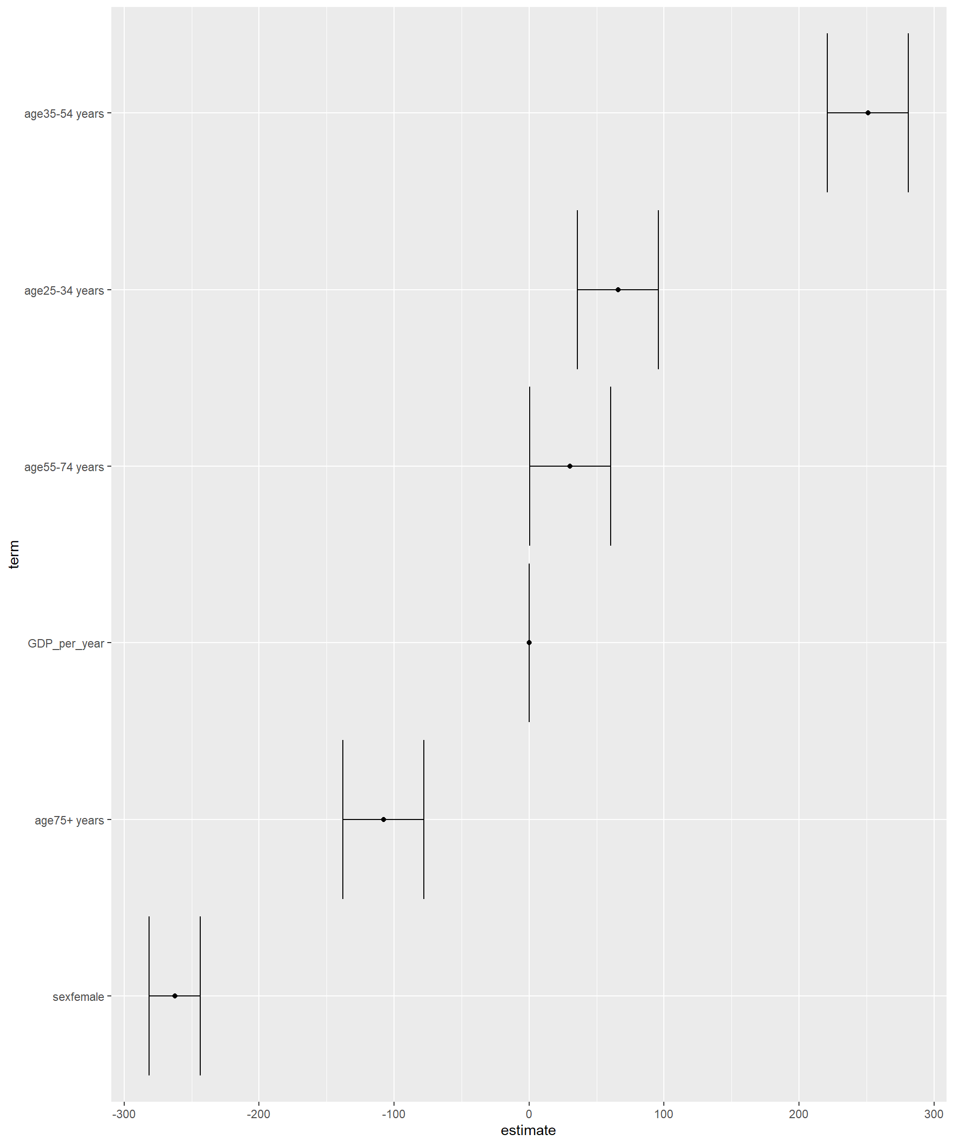
tidy(anova(model2)) %>%
  mutate(Unique = sumsq / sum(sumsq))
## # A tibble: 4 x 7
## term df sumsq meansq statistic p.value Unique
## <chr> <int> <dbl> <dbl> <dbl> <dbl> <dbl>
## 1 GDP_per_year 1 71814. 71814. 10.3 1.50e- 3 0.00630
## 2 age 4 4108872. 1027218. 147. 9.14e-69 0.361
## 3 sex 1 5167969. 5167969. 739. 4.05e-82 0.453
## 4 Residuals 293 2047900. 6989. NA NA 0.180Similar pattern in Australia. Men aged 35 - 54 years old have the highest suicide rate.
age_group_35_54 <- suicide_df %>%
  group_by(country, year, age) %>%
 filter(age %in% "35-54 years") %>%
  summarise(Num = sum(No_of_Suicides))


age_group_35_54 %>%
  filter(country %in% "Australia") %>%
ggplot() +
 aes(x = year, y = Num) +
 geom_point(size = 2, colour = "#0c4c8a") +
  geom_line() +
  labs(title = "Total Suicides in Australia 1985 to 2015",
         subtitle = "Age Group 35 to 54 Years Old",
       x = "Year",
       y = "Number of Suicides") +
  theme(axis.text.x = element_text(angle = 90, hjust = 1))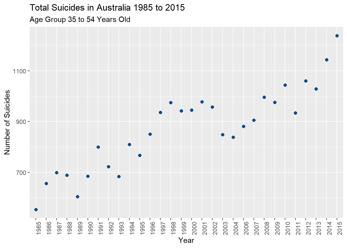
Aaron Willcox
Student
Interests include data wrangling with R and research into neurodevelopmental disorders particularly adult ADHD.