Oceanographic Wave Measuring
This is a simple graphical display of a dataset with wave data from Queensland Australia.
library(tidyverse)
library(lubridate)
library(hrbrthemes)
This dataset contains Measured/Calculated wave parameters. Measured and derived wave data from data collected by oceanographic wave measuring buoys anchored at Mooloolaba. Coverage period: 30 months.
Acknowledgements This data comes from Queensland Government Data - https://data.qld.gov.au/dataset
Date/TimeDate
- Hs Significant wave height, an average of the highest third of the waves in a record
- Hmax The maximum wave height in the record
- Tz The zero upcrossing wave period
- Tp The peak energy wave period
- Peak Direction Direction (related to true north) from which the peak period waves are coming from
- SST Approximation of sea surface temperature
waves_df <-  read_csv("data/Coastal Data System - Waves (Mooloolaba) 01-2017 to 06 - 2019.csv")

# The date format is mixed so some are mdy and other dmy
# Which we will separate out below
waves_df$`Date/Time` <- parse_date_time(waves_df$`Date/Time`, c("dmyHMS", "mdyHMS"), truncated = 3) # Change the date format


waves_df <- separate(waves_df, 'Date/Time', into = c("year", "month", "day"), sep = "-") # Separate out the year month and day


waves_df <- separate(waves_df, 'day', into = c("day", "time"), sep = " ") # separate out the day and time

head(waves_df)
## # A tibble: 6 x 10
## year month day time Hs Hmax Tz Tp `Peak Direction`
## <chr> <chr> <chr> <chr> <dbl> <dbl> <dbl> <dbl> <dbl>
## 1 2017 01 01 00:0~ -99.9 -99.9 -99.9 -99.9 -99.9
## 2 2017 01 01 00:3~ 0.875 1.39 4.42 4.51 -99.9
## 3 2017 01 01 01:0~ 0.763 1.15 4.52 5.51 49
## 4 2017 01 01 01:3~ 0.77 1.41 4.58 5.65 75
## 5 2017 01 01 02:0~ 0.747 1.16 4.51 5.08 91
## 6 2017 01 01 02:3~ 0.718 1.61 4.61 6.18 68
## # ... with 1 more variable: SST <dbl>Average Wave Height for 2017 to 2019 for each month
waves_df %>%
  group_by(year, month) %>%
  summarise(Ave_wave_height = mean(Hs)) %>%
  ggplot(aes(x = month, y = Ave_wave_height)) +
  geom_point(size = 2.2) +
  geom_line(aes(x = month, y = Ave_wave_height)) +
  facet_wrap(~year) +
  theme_bw()+
  theme(axis.text.x = element_text(angle = 90, hjust = 1))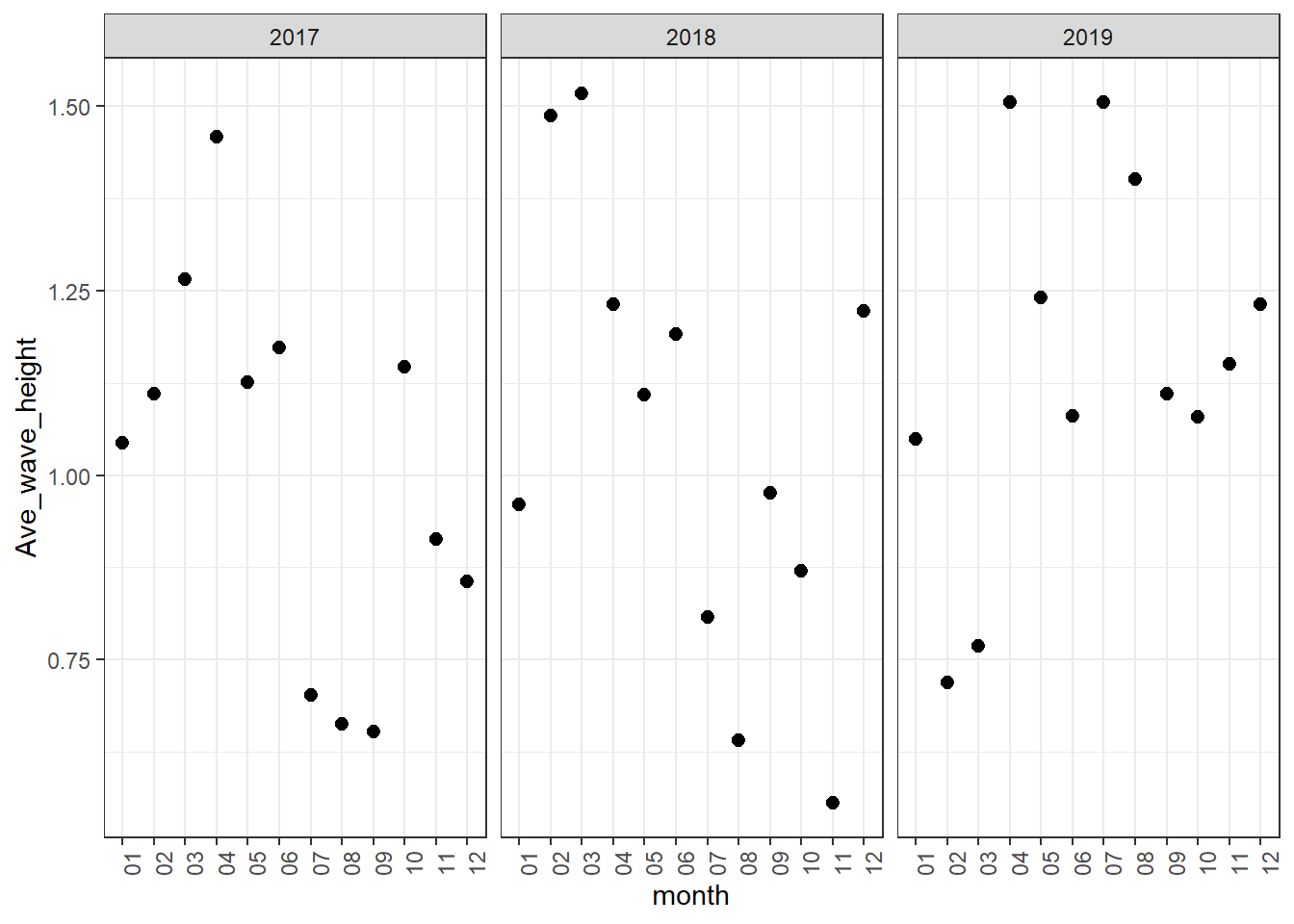
waves_df %>%
  group_by(year, month) %>%
  summarise(Mean = mean(Hs)) %>%
ggplot(aes(x = month, y = Mean, group = year)) +
  geom_line(aes(color = year), size = 1) +
  theme_ft_rc() +
  xlab("Month") +
  ylab("Mean Wave Height") +
  ggtitle("Average Wave Height 2017 to 2019")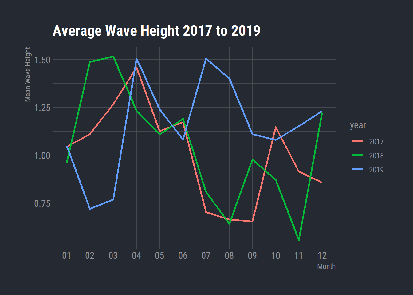
Correlations between variables
waves_cor <- waves_df %>% select(5:10)

waves_cor <- cor(waves_cor)

corrplot::corrplot(waves_cor, is.corr = FALSE)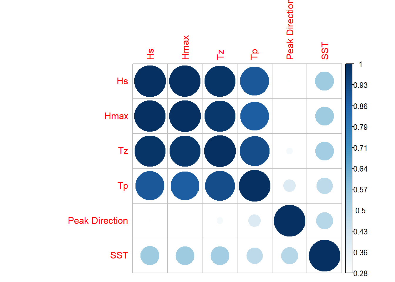
Aaron Willcox
Student
Interests include data wrangling with R and research into neurodevelopmental disorders particularly adult ADHD.