OSL Workshop Solomons Paradox
Does reasoning about personal problems improve with psychological distance?
STUDY DESCRIPTION
Solomon’s paradox describes the tendency for people to reason more wisely about other people’s problems compared to their own. One potential explanation for this paradox is that people tend to view other people’s problems from a more psychologically distant perspective, whereas they view their own problems from a psychologically immersed perspective . For example, imagine two friends, Beth and Zoe, are discussing Zoe’s relationship problems. Beth’s distance allows her to see that Zoe’s relationship is doomed, so she can offer her friend sage advice for how to proceed with her relationship. Zoe’s immersion in her own relationship may lead her to have a hard time reasoning wisely, because she may be worried that she will need to find a new apartment if she breaks up with her boyfriend.
What if, however, Zoe was able to take a more psychologically distanced perspective when contemplating her relationship problems? Would she exhibit a higher level of wisdom, similar to what Beth was able to show? To test this possibility, Grossmann and Kross (2014) asked romantically-involved participants to think about a situation in which their partner cheated on them ( self condition ) or a friend’s partner cheated on their friend ( other condition ). Participants were also instructed to take a first-person perspective ( immersed condition ) by using pronouns such as I and me, or a third-person perspective ( distanced condition ) by using pronouns such as he and her.
Participants were 120 university students who were involved in monogamous, heterosexual romantic relationships, and participants were randomly assigned to condition. After contemplating the infidelity scenario described above with the assigned perspective, participants responded to various questions designed to assess wise reasoning.
Grossmann, I., & Kross, E. (2014). Exploring Solomon’s paradox: Self-distancing eliminates self-other asymmetry in wise reasoning about close relationships in younger and older adults. Psychological Science, 25, 1571-1580.
Given the context of this study, a dimension that could have been explored more was that of how wisdom differs to that of intelligence. In that inteliigence is more applied and wisdom is the ability to learn from an experience.
ANAYSIS
- Open the data file (called Grossmann and Kross 2014 Study 2). Explore the data file. Note, you will not analyze all of these variables. Try to find the variables that are relevant to the study description above.
library(car)
library(dplyr)
library(psych)
library(ggplot2)
library(knitr)
library(pander)

Psych_dist_df <- read.csv("data/Grossman and Kross 2014 Study 2.csv")- Conduct a one-way ANOVA to determine if there is a significant difference between the conditions on wisdom.
Conditions: DV: Wise Reasoning
# Use the names() function to print out the list of variable names
#names(Psych_dist_df)
# We are interested in the conditions and wisdom variables
# so we can use dplyr to select these and print a table to look at
# Can see some NA cases
#complete.cases(Psych_dist_df)

df <- Psych_dist_df[complete.cases(Psych_dist_df), ] # remove cases with NA and subset to new dataframe
df <- select(df, CONDITION, WISDOM) # filter out other variables and only use ones of interest
Descriptives
Descriptives <- select(df, CONDITION, WISDOM) %>%
  group_by(CONDITION) %>%
  summarise(count = n()
            ,mean = mean(WISDOM)
            ,sd = sd(WISDOM))

# viewing the dataframe shows that the CONDITION is currently treated as an INT so we will
# convert this to a factor with label names for clarity
df$CONDITION <- factor(df$CONDITION, labels = c("Self_immersed", "Self_dist", "other_immersed", "other_dist") ) # convert the CONDITION int to a factor


ggplot(data = df) +
  aes(x = CONDITION, y = WISDOM) +
  geom_boxplot(fill = "#26828e") +
  labs(title = "Solomon’s paradox",
    x = "Condition",
    y = "Wisdom",
    subtitle = "Subtitle") +
  theme_bw()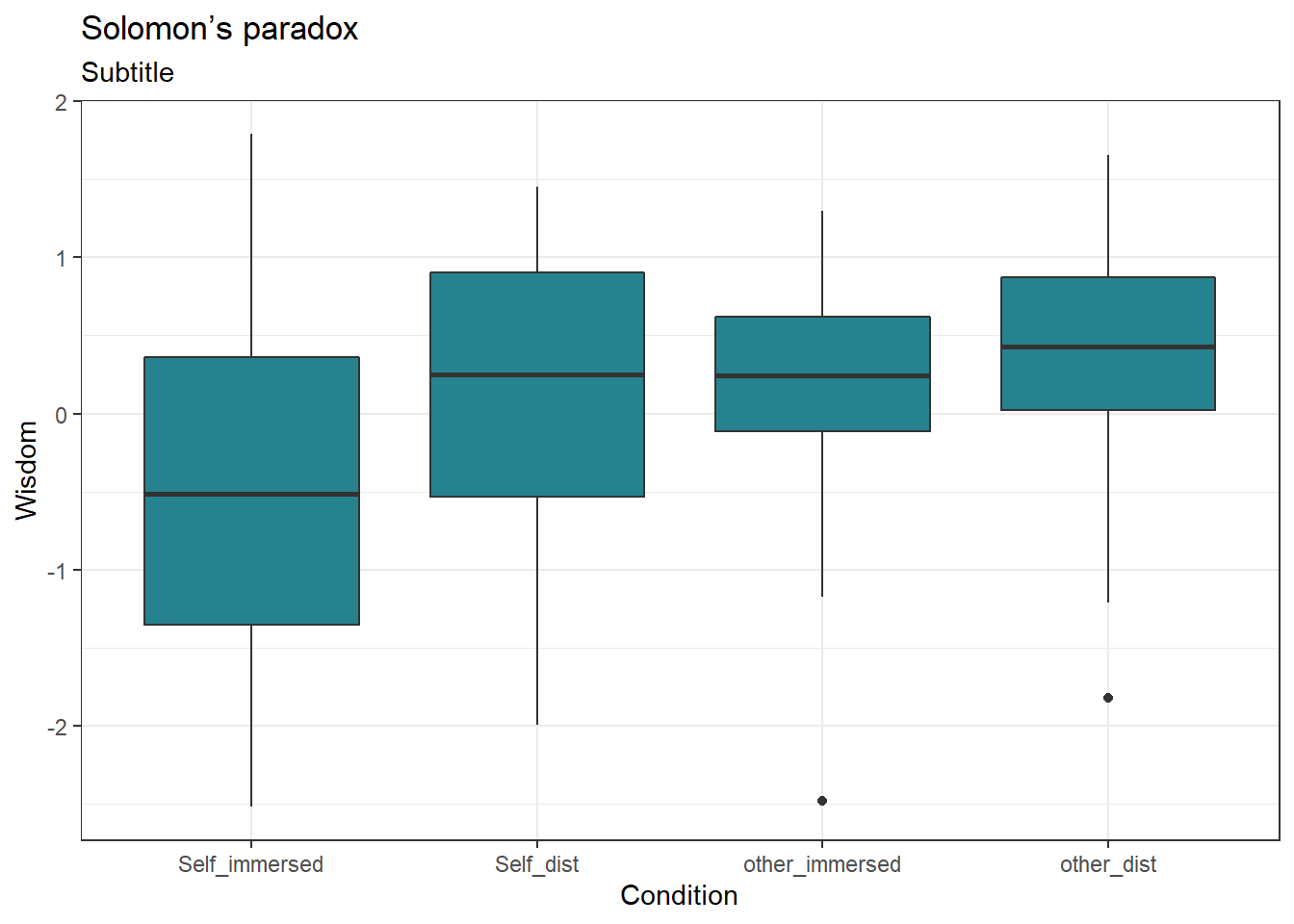
kable(Descriptives) %>% kableExtra::kable_styling()| CONDITION | count | mean | sd |
|---|---|---|---|
| 1 | 31 | -0.5593042 | 1.1660305 |
| 2 | 26 | 0.1220847 | 0.9418065 |
| 3 | 33 | 0.1948435 | 0.7711439 |
| 4 | 25 | 0.3344884 | 0.8129734 |
Visual Analysis
Run ANOVA
anova_model <- lm(WISDOM ~ CONDITION, data = df) #run an anova or lmRun the model through a Anova function
pander(Anova(anova_model, type="III")) # Ue the car package to run the anova| Sum Sq | Df | F value | Pr(>F) | |
|---|---|---|---|---|
| (Intercept) | 9.697 | 1 | 11 | 0.001232 |
| CONDITION | 14.13 | 3 | 5.343 | 0.001783 |
| Residuals | 97.86 | 111 | NA | NA |
Levene’s Test
pander(leveneTest(anova_model)) # tests of homogeniety| Df | F value | Pr(>F) | |
|---|---|---|---|
| group | 3 | 3.581 | 0.01619 |
| 111 | NA | NA |
Using the lm() function from earlier, printing the summary results in contrasts.
pander(summary(anova_model)) # summary.lm gives us each level of the condition| Estimate | Std. Error | t value | Pr(>|t|) | |
|---|---|---|---|---|
| (Intercept) | -0.5593 | 0.1686 | -3.317 | 0.001232 |
| CONDITIONSelf_dist | 0.6814 | 0.2497 | 2.729 | 0.00739 |
| CONDITIONother_immersed | 0.7541 | 0.2348 | 3.211 | 0.001729 |
| CONDITIONother_dist | 0.8938 | 0.2524 | 3.541 | 0.0005833 |
| Observations | Residual Std. Error | Adjusted | |
|---|---|---|---|
| 115 | 0.9389 | 0.1262 | 0.1026 |
Box plot
ggplot(data = df
       , aes(x = CONDITION, y = WISDOM, colour = CONDITION)) +
  geom_boxplot(outlier.colour="red" # the geom_ must be on the same line
               , outlier.shape=16
               , outlier.size=2
, notch=TRUE) 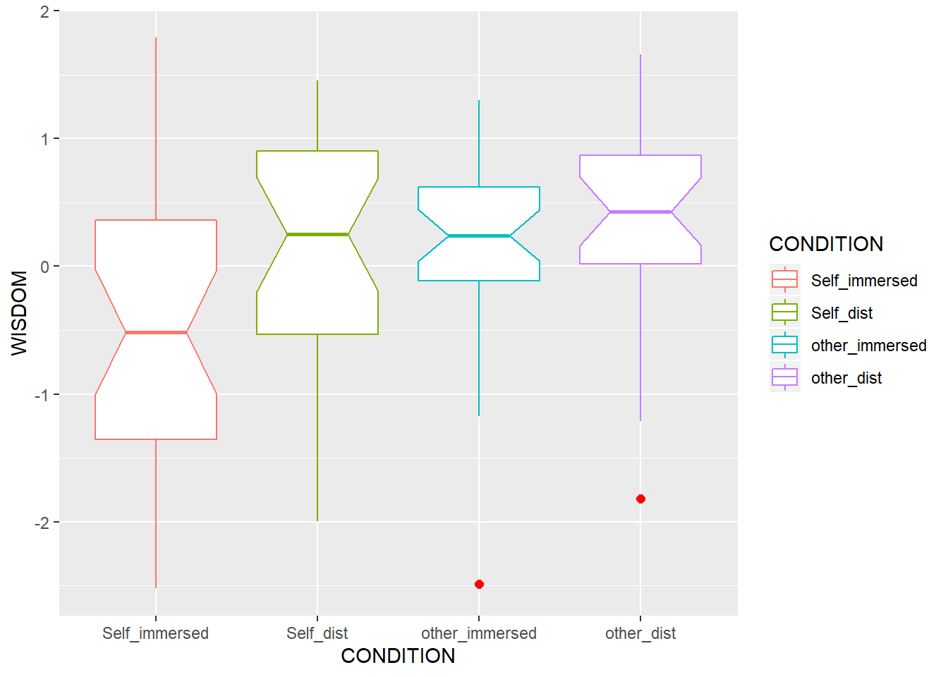
- Next, you want to determine whether the self-immersed condition was significantly lower in wisdom, relative to the other-immersed and other-distanced condition. Conduct a planned contrast to test the typical Solomon’s paradox effect.
# planned contrasts
c1 <- c(2, 0, -1, -1)
planned_contrasts <-c1
contrasts(df$CONDITION) <- planned_contrasts
model1 <- aov(WISDOM ~ CONDITION, data = df)
Anova(model1, type = "III")## Anova Table (Type III tests)
##
## Response: WISDOM
## Sum Sq Df F value Pr(>F)
## (Intercept) 0.060 1 0.0682 0.794390
## CONDITION 14.131 3 5.3432 0.001783 **
## Residuals 97.855 111
## ---
## Signif. codes: 0 '***' 0.001 '**' 0.01 '*' 0.05 '.' 0.1 ' ' 1summary.aov(model1, split = list(CONDITION = list("Self_immersed" = 1, "Self_dist" = 2, "other_immersed" = 3, "other_dist" = 4)))## Df Sum Sq Mean Sq F value Pr(>F)
## CONDITION 3 14.13 4.710 5.343 0.00178 **
## CONDITION: Self_immersed 1 13.47 13.468 15.277 0.00016 ***
## CONDITION: Self_dist 1 0.66 0.660 0.749 0.38875
## CONDITION: other_immersed 1 0.00 0.003 0.004 0.95210
## CONDITION: other_dist 1
## Residuals 111 97.86 0.882
## ---
## Signif. codes: 0 '***' 0.001 '**' 0.01 '*' 0.05 '.' 0.1 ' ' 1- Now, you want to show that taking a distant perspective increases wisdom relative to taking an immersed perspective when dealing with one’s own problems. Conduct a planned contrast to determine whether self-distancing results in significantly higher levels of wisdom, relative to self-immersion.
c2 <- c(1, -1, 0, 0) # self distance vs self immursion
planned_contrasts <-c2
contrasts(df$CONDITION) <- planned_contrasts
model2 <- aov(WISDOM ~ CONDITION, data = df)
Anova(model2, type = "III")## Anova Table (Type III tests)
##
## Response: WISDOM
## Sum Sq Df F value Pr(>F)
## (Intercept) 0.060 1 0.0682 0.794390
## CONDITION 14.131 3 5.3432 0.001783 **
## Residuals 97.855 111
## ---
## Signif. codes: 0 '***' 0.001 '**' 0.01 '*' 0.05 '.' 0.1 ' ' 1summary.aov(model2, split = list(CONDITION = list("Self_immersed" = 1, "Self_dist" = 2, "other_immersed" = 3, "other_dist" = 4)))## Df Sum Sq Mean Sq F value Pr(>F)
## CONDITION 3 14.13 4.710 5.343 0.00178 **
## CONDITION: Self_immersed 1 7.43 7.430 8.428 0.00446 **
## CONDITION: Self_dist 1 2.32 2.317 2.629 0.10780
## CONDITION: other_immersed 1 4.38 4.384 4.973 0.02775 *
## CONDITION: other_dist 1
## Residuals 111 97.86 0.882
## ---
## Signif. codes: 0 '***' 0.001 '**' 0.01 '*' 0.05 '.' 0.1 ' ' 1- You also want to determine whether distancing vs. immersion increases wisdom when contemplating other people’s problems. Conduct a planned contrast to compare the other-distance vs. other-immersed conditions.
c3 <- c(0, 0, 1, -1) # other immersed vs other distance
planned_contrasts <-c3
contrasts(df$CONDITION) <- planned_contrasts
model3 <- aov(WISDOM ~ CONDITION, data = df)
Anova(model3, type = "III")## Anova Table (Type III tests)
##
## Response: WISDOM
## Sum Sq Df F value Pr(>F)
## (Intercept) 0.060 1 0.0682 0.794390
## CONDITION 14.131 3 5.3432 0.001783 **
## Residuals 97.855 111
## ---
## Signif. codes: 0 '***' 0.001 '**' 0.01 '*' 0.05 '.' 0.1 ' ' 1summary.aov(model3, split = list(CONDITION = list("Self_immersed" = 1, "Self_dist" = 2, "other_immersed" = 3, "other_dist" = 4)))## Df Sum Sq Mean Sq F value Pr(>F)
## CONDITION 3 14.13 4.710 5.343 0.001783 **
## CONDITION: Self_immersed 1 0.07 0.068 0.077 0.781773
## CONDITION: Self_dist 1 1.77 1.769 2.007 0.159391
## CONDITION: other_immersed 1 12.29 12.294 13.946 0.000299 ***
## CONDITION: other_dist 1
## Residuals 111 97.86 0.882
## ---
## Signif. codes: 0 '***' 0.001 '**' 0.01 '*' 0.05 '.' 0.1 ' ' 1- Finally, you want to test whether self-distancing eliminates the increased wisdom typically found in reasoning about others. Conduct a planned comparison to determine whether the self-distanced condition is significantly different from the other-immersed and other-distanced conditions.
c4 <- c(0, 2, -1, -1) # self dist vs other immersed & other dist
planned_contrasts <-c4
contrasts(df$CONDITION) <- planned_contrasts
model4 <- aov(WISDOM ~ CONDITION, data = df)
Anova(model4, type = "III")## Anova Table (Type III tests)
##
## Response: WISDOM
## Sum Sq Df F value Pr(>F)
## (Intercept) 0.060 1 0.0682 0.794390
## CONDITION 14.131 3 5.3432 0.001783 **
## Residuals 97.855 111
## ---
## Signif. codes: 0 '***' 0.001 '**' 0.01 '*' 0.05 '.' 0.1 ' ' 1summary.aov(model4, split = list(CONDITION = list("Self_immersed" = 1, "Self_dist" = 2, "other_immersed" = 3, "other_dist" = 4)))## Df Sum Sq Mean Sq F value Pr(>F)
## CONDITION 3 14.13 4.710 5.343 0.00178 **
## CONDITION: Self_immersed 1 0.44 0.438 0.496 0.48260
## CONDITION: Self_dist 1 5.48 5.476 6.212 0.01417 *
## CONDITION: other_immersed 1 8.22 8.218 9.322 0.00283 **
## CONDITION: other_dist 1
## Residuals 111 97.86 0.882
## ---
## Signif. codes: 0 '***' 0.001 '**' 0.01 '*' 0.05 '.' 0.1 ' ' 1Prepare an APA-style results section to describe each of the analyses conducted above.
Generate a bar graph to depict the results for the one-way ANOVA. Don’t forget to include error bars that reflect the +/- 1 standard error of the mean.
ggplot(df, aes(CONDITION, WISDOM))+
  stat_boxplot( aes(CONDITION, WISDOM),
    geom='errorbar', linetype=1, width=0.5)+  #whiskers
  geom_boxplot( aes(CONDITION, WISDOM),outlier.shape=1) +
  stat_summary(fun.y=mean, geom="point", size=2) +
  stat_summary(fun.data = mean_se, geom = "errorbar")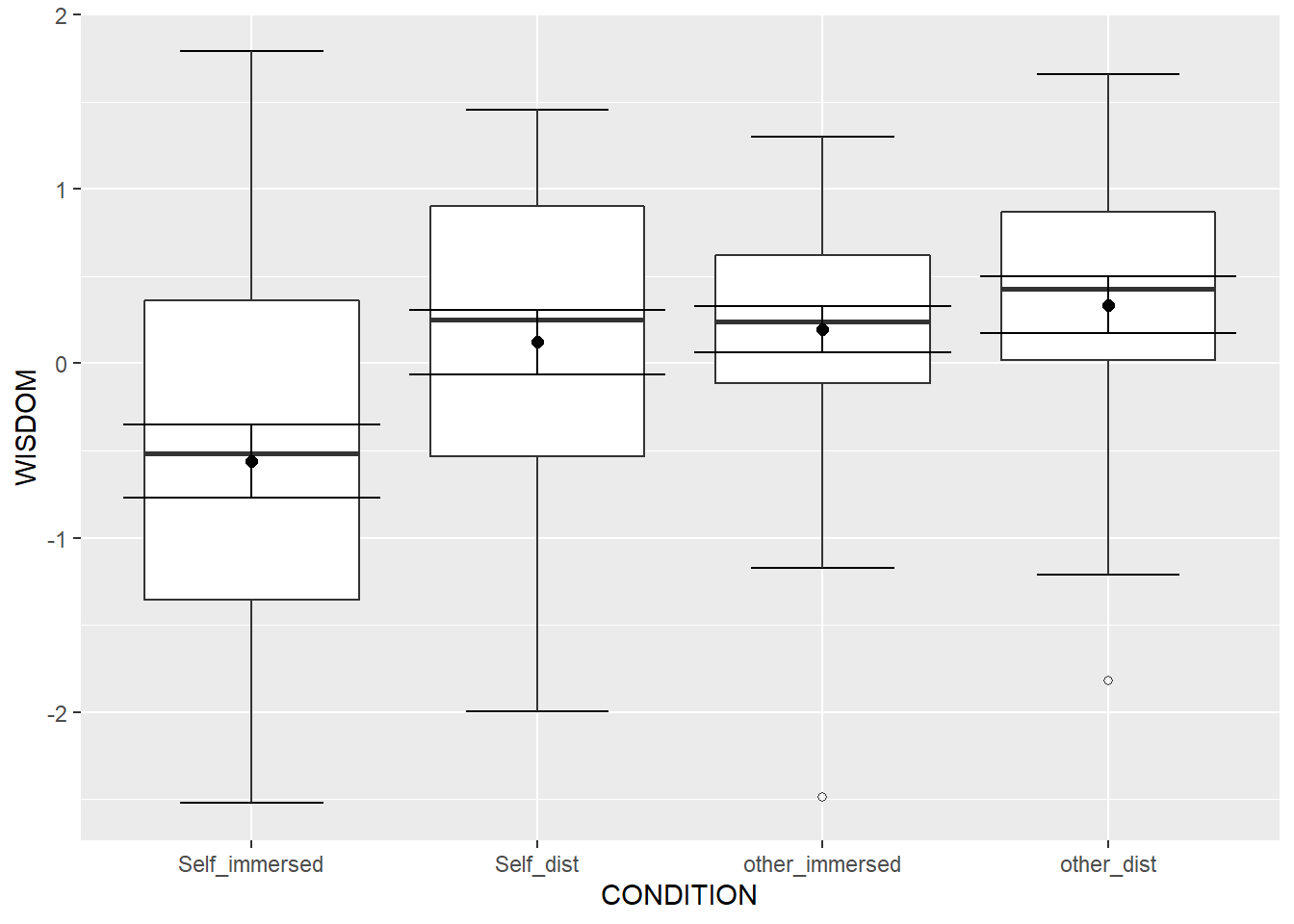
Aaron Willcox
Student
Interests include data wrangling with R and research into neurodevelopmental disorders particularly adult ADHD.