PCA on US Nutrition
A quick walk through of running a PCA on US nutrition and the use of a couple of different packages in R, to display information graphically.
library(tidyverse)
library(corrplot)
library(cowplot)
library(hrbrthemes)
Information
The following dataset froms from the Nutrient database in the United States
This is from the now outdated SR27. It is also created from the full database. The “abbreviated file” in SR28 is more up to date than this data and contains more nutrients than we provide here. See https://data.world/awram/food-nutritional-values
The columns in US RDA are created using data from Dietary Reference Intakes: The Essential Guide to Nutrient Requirements available from the National Academies Press at http://www.nap.edu/catalog/11537.html
Data Each record is for 100 grams.
The columns are mostly self-explanatory. The nutrient columns end with the units, so:
Nutrient_g is in grams Nutrient_mg is in milligrams Nutrient_mcg is in micrograms Nutrient_USRDA is in percentage of US Recommended Daily Allows (e.g. 0.50 is 50%) Note that not every available RDA value in the text was used. For instance, the US RDA for Iron varies significantly by age and sex, so I deemed it easier to just leave out RDA information for Iron.
# data_df <- read.csv(file = "https://query.data.world/s/iwzl7xgiagpimb2ixfj4fkyztngxs7", stringsAsFactors = FALSE, header = TRUE)

#write.csv(data_df, file = "data/nutrian_df.csv") # write the dataframe to csv

data_df <- read_csv(file = "data/nutrian_df.csv")
Running a Principle Componant Analysis on the United States Dietry Reference Nutrient Database
The USRDA containts the same information as _mg so these are reduntant and can be removed.
data_df <- data_df %>% select(-contains("_USRDA"))Catagorical Visualisation
data_df$FoodGroup <- factor(data_df$FoodGroup, ordered = is.ordered(data_df$FoodGroup)) # coerce to factor

Foodgroup_cat <- data_df %>% # Group by the food group catagory and count the amont each one occurs
  group_by(FoodGroup) %>%
  summarise(N = n()) %>%
  arrange(N)


Foodgroup_cat$FoodGroup <- str_remove(Foodgroup_cat$FoodGroup, "Products") # Remove the word "products" from the list

ggplot(Foodgroup_cat) +
 aes(x = reorder(FoodGroup, -N), y = N) +
 geom_bar(stat = "identity") +
 coord_flip() +
  labs(title = "Toal Amount of Food Products",
       subtitle = "USDRA",
       x = "Products",
       y = "Frequency") +
  theme_ft_rc()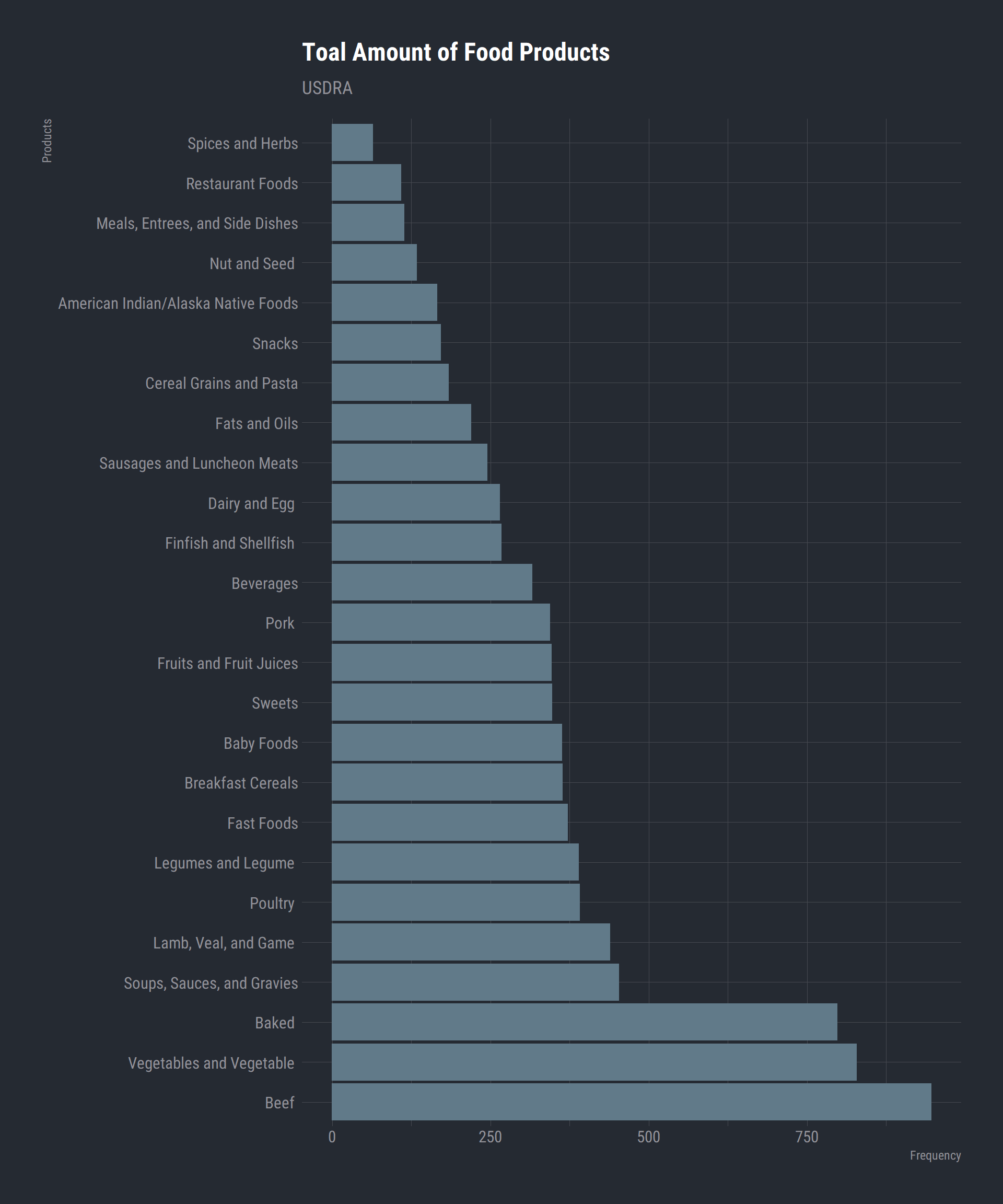
Amount of sugar in grams associated with total energy (k/cals) for each food group
ggplot(data_df) +
aes(x = Sugar_g, y = Energy_kcal, fill = FoodGroup, colour = FoodGroup) +
geom_point(size = 1L) +
scale_fill_hue() +
scale_color_hue() +
labs(x = "Sugar in gram", y = "Energy in k/cals", title = "Amount of Energy from Sugar for each Food Group", subtitle = "Food Groups") +
theme_ft_rc() +
theme(legend.position = "none") +
facet_wrap(vars(FoodGroup), scales = "free_x")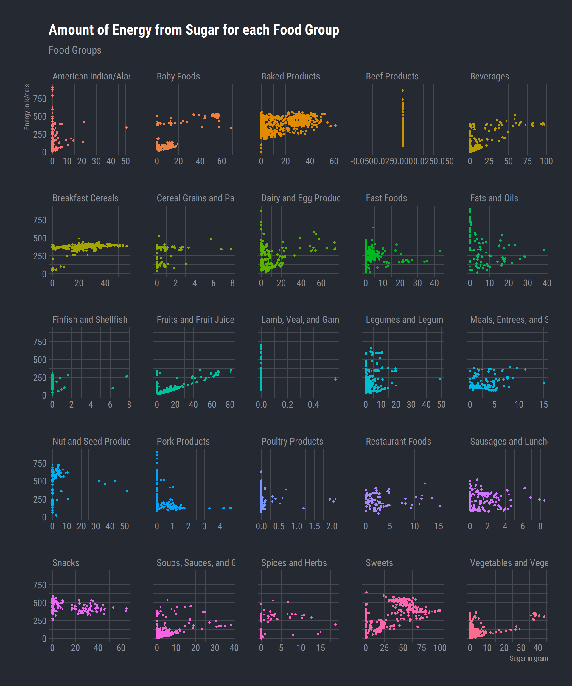 Beef, lamb, veal and game products tend to have very little sugar/energy. Theres a clustering of points in the beverages table
and would assume this would be water or low sugar drinks. Considering this is a database of nutrients based on major food groups, we cant tease out the underlying specifics of the types of drinks or products.
Beef, lamb, veal and game products tend to have very little sugar/energy. Theres a clustering of points in the beverages table
and would assume this would be water or low sugar drinks. Considering this is a database of nutrients based on major food groups, we cant tease out the underlying specifics of the types of drinks or products.
There is some skewness in the data and could do with some transforming but theres no guarentee that it will improve results. Here we will rescale and center the variables with a mean of 0 and a variance of 1. Then run a correlation matrix to visualise the results.
data_df[,9:31] <- sqrt(data_df[,9:31]) # sqrt transform

data_df_rescale <- data_df %>%
  select(9:31) %>%
  scale(center = TRUE)

data_df_corr <- data_df %>% select(9:31)

data_corrr <- cor(data_df_corr)

corrplot(as.matrix(data_corrr), is.corr = FALSE, method = "square", type = "full")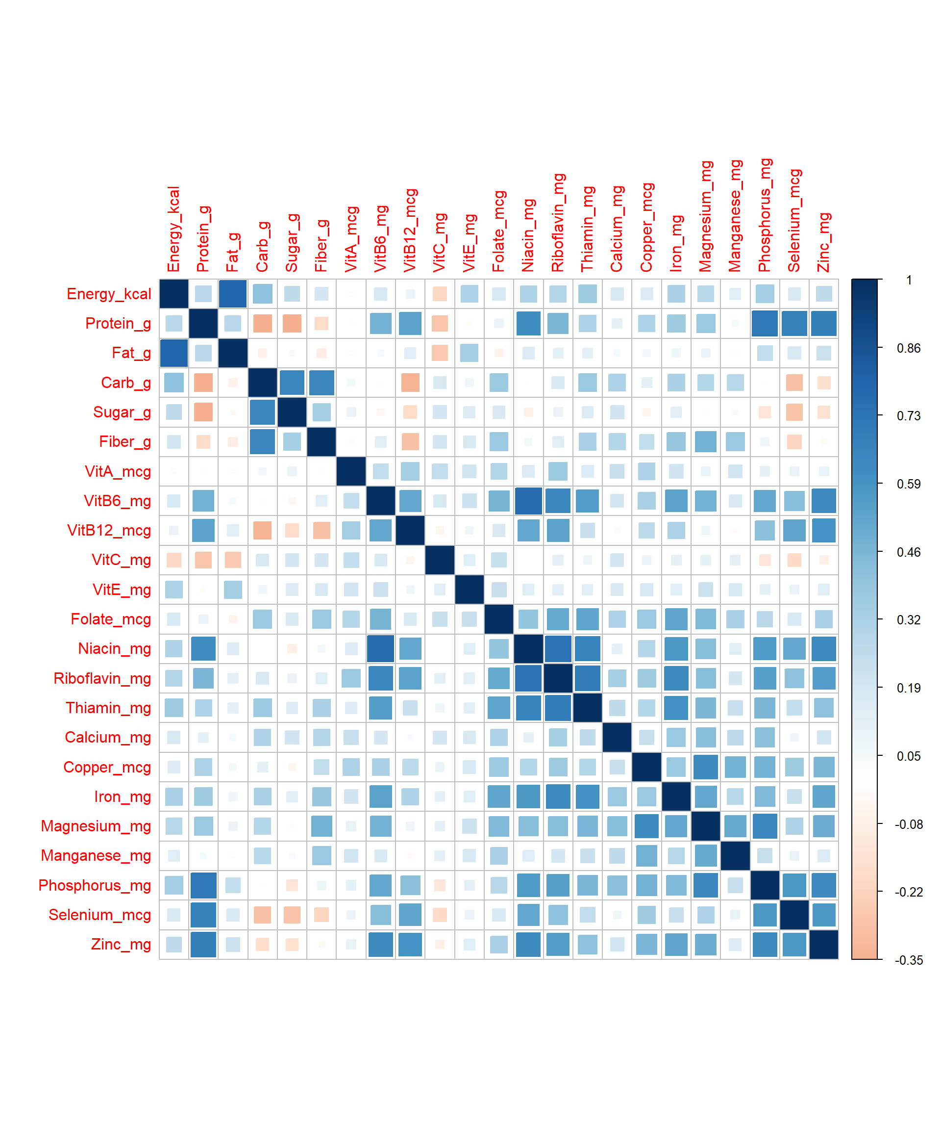
Run a PCA with the default prcomp function in R and run a summary on the object then display a scree plot with eigen vectors:
data_PCA <- prcomp(data_df_rescale)

# print(data_PCA) # Full PCA matrix

summary(data_PCA)
## Importance of components:
## PC1 PC2 PC3 PC4 PC5 PC6
## Standard deviation 2.7035 1.9212 1.42556 1.24459 1.17551 0.96650
## Proportion of Variance 0.3178 0.1605 0.08836 0.06735 0.06008 0.04061
## Cumulative Proportion 0.3178 0.4783 0.56661 0.63396 0.69404 0.73465
## PC7 PC8 PC9 PC10 PC11 PC12
## Standard deviation 0.92451 0.81294 0.77169 0.73023 0.71235 0.68914
## Proportion of Variance 0.03716 0.02873 0.02589 0.02318 0.02206 0.02065
## Cumulative Proportion 0.77182 0.80055 0.82644 0.84963 0.87169 0.89234
## PC13 PC14 PC15 PC16 PC17 PC18
## Standard deviation 0.61955 0.60078 0.55051 0.51154 0.48452 0.46802
## Proportion of Variance 0.01669 0.01569 0.01318 0.01138 0.01021 0.00952
## Cumulative Proportion 0.90903 0.92472 0.93789 0.94927 0.95948 0.96900
## PC19 PC20 PC21 PC22 PC23
## Standard deviation 0.45204 0.4317 0.38515 0.37130 0.18989
## Proportion of Variance 0.00888 0.0081 0.00645 0.00599 0.00157
## Cumulative Proportion 0.97789 0.9860 0.99244 0.99843 1.00000plot(data_PCA, type = "l")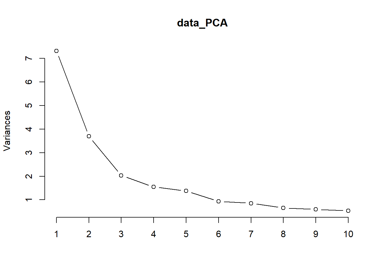
# data_PCA$rotationThe summary method describe the importance of the PCs. The first row describe again the standard deviation associated with each PC. The second row shows the proportion of the variance in the data explained by each component while the third row describe the cumulative proportion of explained variance. We can see there that the first two PCs accounts for more than 47% (0.31+0.16) of the variance of the data. The remaining 53% is shared across PC3 to PC23.
From the plot we can see that factors load the most on PC1 and PC2. The Scree plot also shows us visualy where the components fall off after PC1 and PC2. Use the FactorMineR package to extract more detailed data howver, will use the first 5 components as these tend to load the most on the components (69%).
library(FactoMineR)

data_PCA_all <- PCA(data_df_rescale, ncp  = 2, graph = TRUE)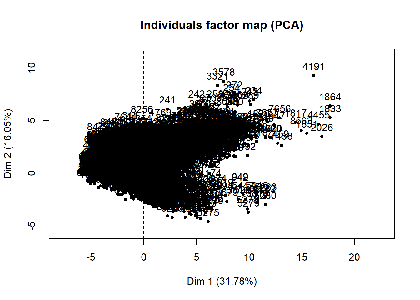
data_PCA_all$eig #eigen values, percent of varaince and cumulative percentage## eigenvalue percentage of variance
## comp 1 7.30899804 31.7782524
## comp 2 3.69088747 16.0473368
## comp 3 2.03221880 8.8357339
## comp 4 1.54900652 6.7348110
## comp 5 1.38181755 6.0079024
## comp 6 0.93411330 4.0613622
## comp 7 0.85472741 3.7162061
## comp 8 0.66087037 2.8733494
## comp 9 0.59551138 2.5891799
## comp 10 0.53323222 2.3184010
## comp 11 0.50743683 2.2062471
## comp 12 0.47491477 2.0648468
## comp 13 0.38384585 1.6688950
## comp 14 0.36094051 1.5693065
## comp 15 0.30306178 1.3176599
## comp 16 0.26167535 1.1377189
## comp 17 0.23475988 1.0206951
## comp 18 0.21904338 0.9523625
## comp 19 0.20433782 0.8884253
## comp 20 0.18634147 0.8101803
## comp 21 0.14834034 0.6449580
## comp 22 0.13786150 0.5993978
## comp 23 0.03605747 0.1567716
## cumulative percentage of variance
## comp 1 31.77825
## comp 2 47.82559
## comp 3 56.66132
## comp 4 63.39613
## comp 5 69.40404
## comp 6 73.46540
## comp 7 77.18160
## comp 8 80.05495
## comp 9 82.64413
## comp 10 84.96254
## comp 11 87.16878
## comp 12 89.23363
## comp 13 90.90252
## comp 14 92.47183
## comp 15 93.78949
## comp 16 94.92721
## comp 17 95.94790
## comp 18 96.90027
## comp 19 97.78869
## comp 20 98.59887
## comp 21 99.24383
## comp 22 99.84323
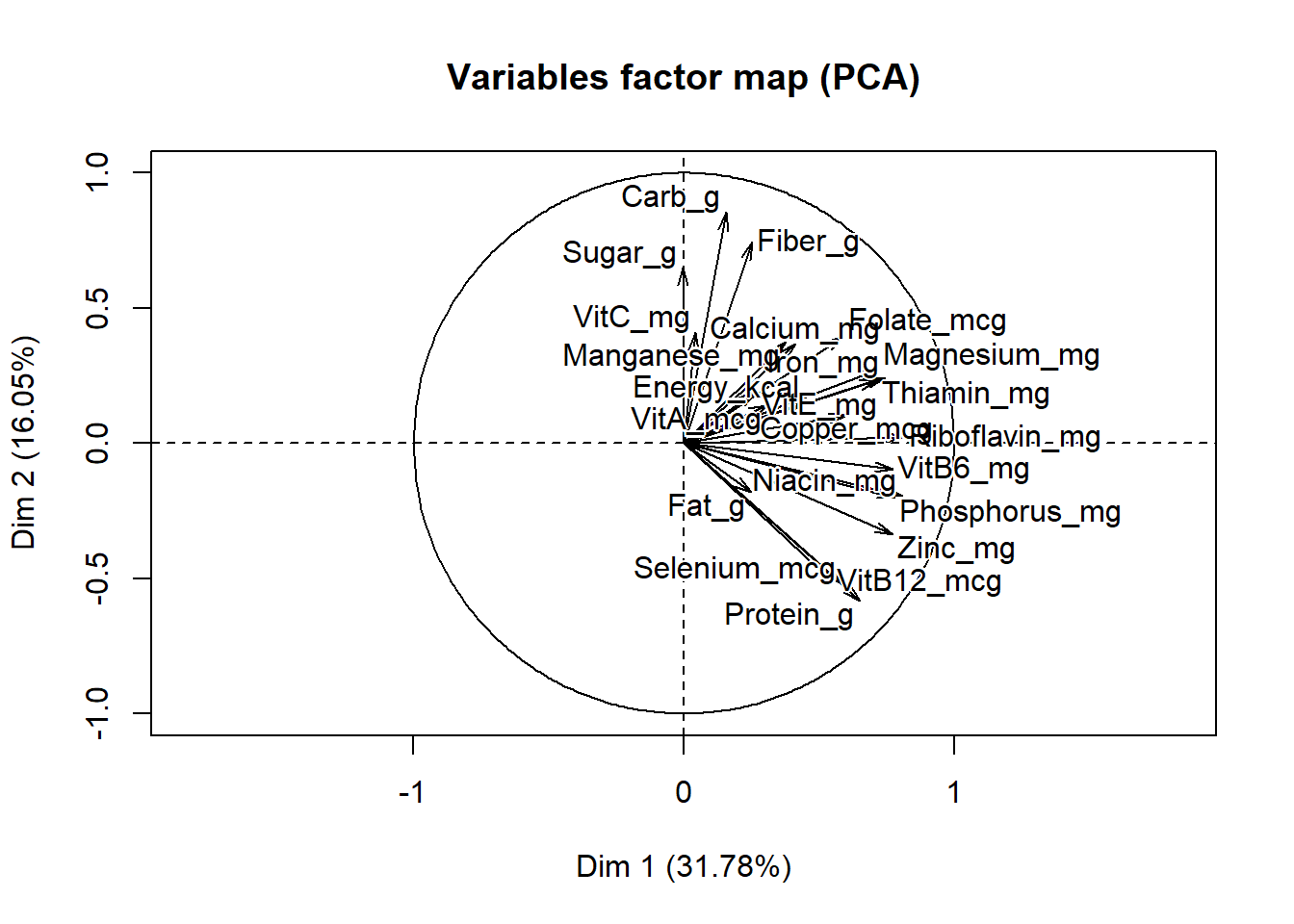
## comp 23 100.00000data_PCA_all$var$coord # correlations betwewen variables and PCs## Dim.1 Dim.2
## Energy_kcal 0.448057415 0.15136222
## Protein_g 0.652364089 -0.58221037
## Fat_g 0.249819599 -0.18205001
## Carb_g 0.158105970 0.85394168
## Sugar_g -0.004775929 0.65028120
## Fiber_g 0.251606686 0.74499520
## VitA_mcg 0.307971932 0.13860307
## VitB6_mg 0.772433885 -0.09606918
## VitB12_mcg 0.547003966 -0.50985668
## VitC_mg 0.043794729 0.40875652
## VitE_mg 0.267686499 0.19364742
## Folate_mcg 0.591668201 0.39794955
## Niacin_mg 0.807997717 -0.19436594
## Riboflavin_mg 0.812785526 0.02361212
## Thiamin_mg 0.716976586 0.23537745
## Calcium_mg 0.413959708 0.36642193
## Copper_mcg 0.601837302 0.10344439
## Iron_mg 0.743808829 0.24374640
## Magnesium_mg 0.716083740 0.27292863
## Manganese_mg 0.376447365 0.37623498
## Phosphorus_mg 0.780578918 -0.20048927
## Selenium_mcg 0.584192531 -0.52000769
## Zinc_mg 0.773393089 -0.33565448When variables correlate strongly together they all converge on the same component. A simple method to extract the results, for variables, from a PCA output is to use the function get_pca_var() [factoextra package]. This function provides a list of matrices containing all the results for the active variables (coordinates, correlation between variables and axes, squared cosine and contributions)
This provides a nicer toolset to work with and display the PCA data:
library(factoextra)

# a more colourful visual representation of the variables and where they converge on a component.
fviz_pca_var(data_PCA_all
             , col.var = "cos2"
             , gradient.cols = c("#00AFBB", "#E7B800", "#FC4E07")
             , repel = TRUE) # Avoid text overlapping)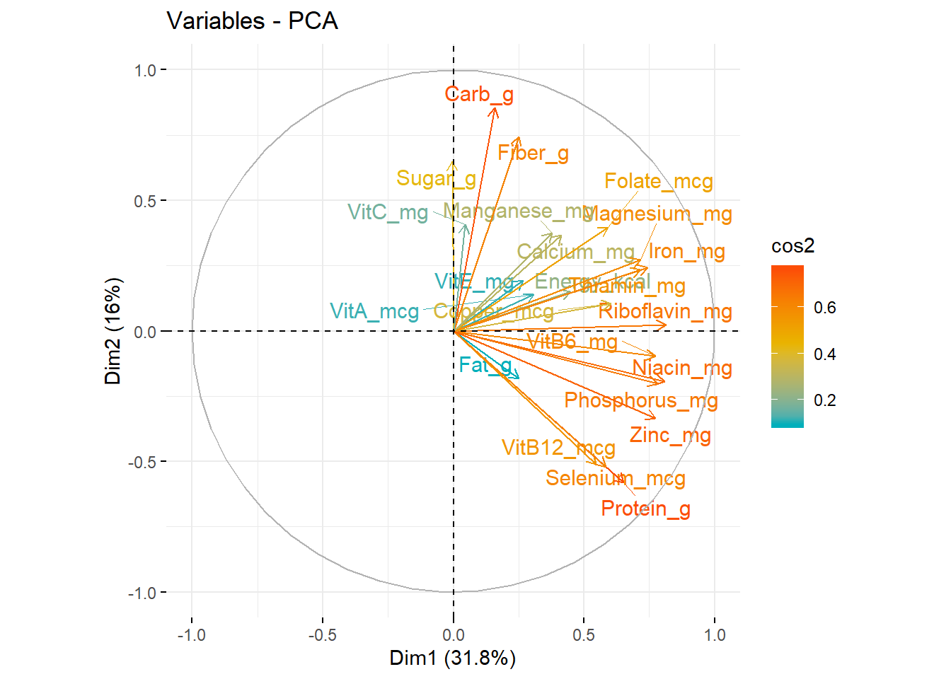
get_eig(data_PCA_all) # display the eigen values, dimensions and variance## eigenvalue variance.percent cumulative.variance.percent
## Dim.1 7.30899804 31.7782524 31.77825
## Dim.2 3.69088747 16.0473368 47.82559
## Dim.3 2.03221880 8.8357339 56.66132
## Dim.4 1.54900652 6.7348110 63.39613
## Dim.5 1.38181755 6.0079024 69.40404
## Dim.6 0.93411330 4.0613622 73.46540
## Dim.7 0.85472741 3.7162061 77.18160
## Dim.8 0.66087037 2.8733494 80.05495
## Dim.9 0.59551138 2.5891799 82.64413
## Dim.10 0.53323222 2.3184010 84.96254
## Dim.11 0.50743683 2.2062471 87.16878
## Dim.12 0.47491477 2.0648468 89.23363
## Dim.13 0.38384585 1.6688950 90.90252
## Dim.14 0.36094051 1.5693065 92.47183
## Dim.15 0.30306178 1.3176599 93.78949
## Dim.16 0.26167535 1.1377189 94.92721
## Dim.17 0.23475988 1.0206951 95.94790
## Dim.18 0.21904338 0.9523625 96.90027
## Dim.19 0.20433782 0.8884253 97.78869
## Dim.20 0.18634147 0.8101803 98.59887
## Dim.21 0.14834034 0.6449580 99.24383
## Dim.22 0.13786150 0.5993978 99.84323
## Dim.23 0.03605747 0.1567716 100.00000fviz_eig(data_PCA_all) # screeplot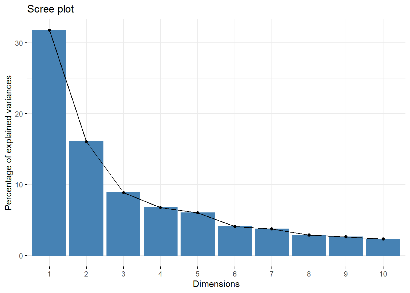
corrplot(data_PCA_all$var$cor, is.corr=FALSE) 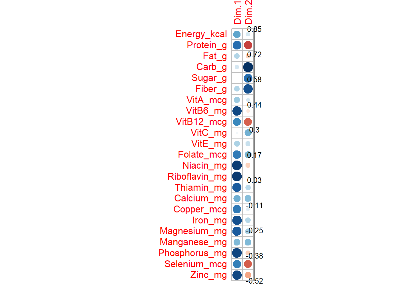
fviz_contrib(data_PCA_all, choice = "var", axes = 1:2, top = 10)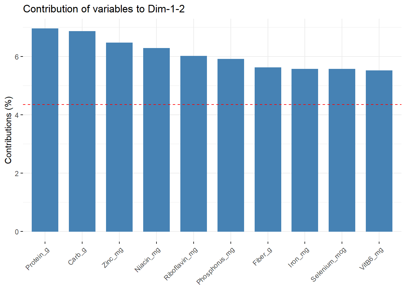
Finally, with the Ggforce package we are able to plot multiple components from a PCA analysis against each other component:
library(ggforce)


pca_grid <- as.data.frame(data_PCA$rotation)

# Since the first ttwo compomnents make up most of the variance explain will add the
# 5 to make up 77% of the components for this example


ggplot(pca_grid[,1:7], aes(x = .panel_x, y = .panel_y)) +
  geom_point(alpha = 0.9, shape = 16, size = 0.5) +
  geom_autodensity() +
  geom_density2d() +
  facet_matrix(vars(everything()), layer.diag = 2, layer.upper = 3,
               grid.y.diag = FALSE)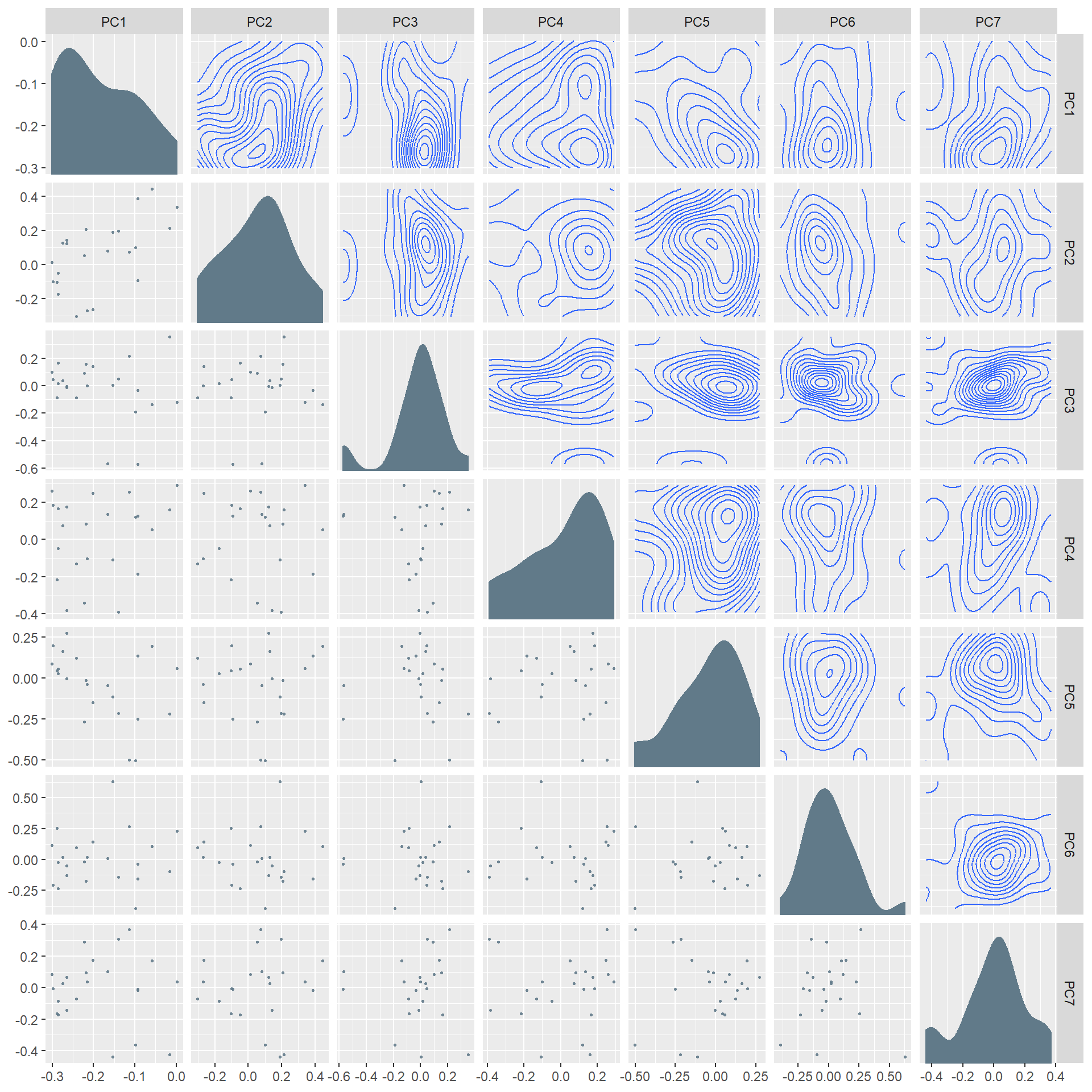
Aaron Willcox
Student
Interests include data wrangling with R and research into neurodevelopmental disorders particularly adult ADHD.