Global Mortality Rates
Global Mortality Rates
The following dataset is from the Tidy Tuesday https://github.com/rfordatascience/tidytuesday/tree/master/data/2018/2018-04-16.
library(tidyverse)
library(hrbrthemes) # custom dark theme from hrbrpackage
global_mort <- read_csv(file = "data/global_mortality.csv", col_names = TRUE) # import dataset into object
global_mort$country <- as.factor(global_mort$country) # Change character to factors
global_mort$country_code <- as.factor(global_mort$country_code)
global_mort$year <- as.factor(global_mort$year)Graphical Display of mortality rates in Australia from 1990 to 2016
df <- global_mort %>%
  group_by(country, year) %>%
  pivot_longer(cols = c(4:35))

df$name <- factor(df$name)


df %>%
  filter("Australia" %in% country) %>%
  #filter("Alcohol disorders (%)" == name) %>%
  #top_n(-15) %>%
ggplot(aes(x = year, y = value, group = name)) +
 geom_line(aes(color = name), size = 1) +
 labs(x = "Year", y = "Percentage (%)", title = "Australian Mortality Rates", subtitle = "1990 to 2016") +
  theme_ft_rc() +
  theme(axis.text.x = element_text(size=10, angle=45)) +
  scale_y_percent()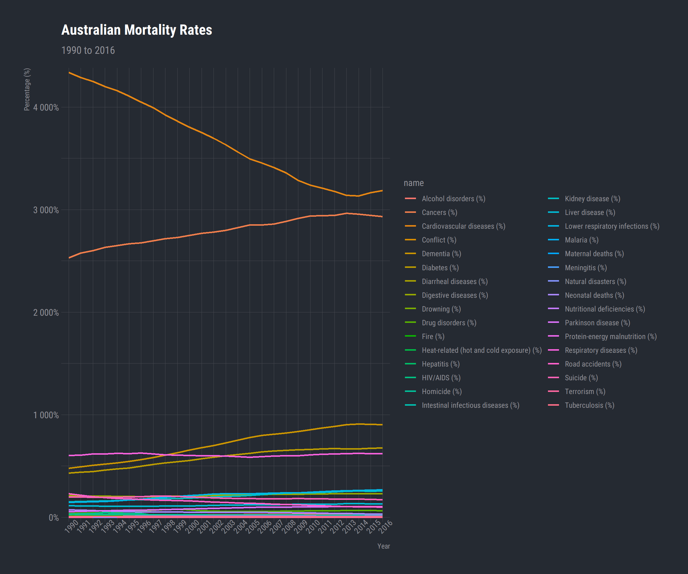
# ggplotly(p)

df %>%
  filter("Australia" %in% country) %>%
  group_by(year, name) %>%
filter(name == "Alcohol disorders (%)")## # A tibble: 27 x 5
## # Groups: year, name [27]
## country country_code year name value
## <fct> <fct> <fct> <fct> <dbl>
## 1 Australia AUS 1990 Alcohol disorders (%) 0.216
## 2 Australia AUS 1991 Alcohol disorders (%) 0.215
## 3 Australia AUS 1992 Alcohol disorders (%) 0.213
## 4 Australia AUS 1993 Alcohol disorders (%) 0.216
## 5 Australia AUS 1994 Alcohol disorders (%) 0.218
## 6 Australia AUS 1995 Alcohol disorders (%) 0.225
## 7 Australia AUS 1996 Alcohol disorders (%) 0.225
## 8 Australia AUS 1997 Alcohol disorders (%) 0.232
## 9 Australia AUS 1998 Alcohol disorders (%) 0.234
## 10 Australia AUS 1999 Alcohol disorders (%) 0.244
## # ... with 17 more rowsAustralia <- global_mort %>%
group_by(country, year) %>%
arrange(year) %>%
filter(country == "Australia")
ggplot(Australia) +
aes(x = year, weight = `Cardiovascular diseases (%)`) +
geom_bar(fill = ft_cols$blue) +
labs(x = "", y = "Amount %", title = "Cardiovascular Disease in Australia", subtitle = "1990 to 2016") +
theme_ft_rc()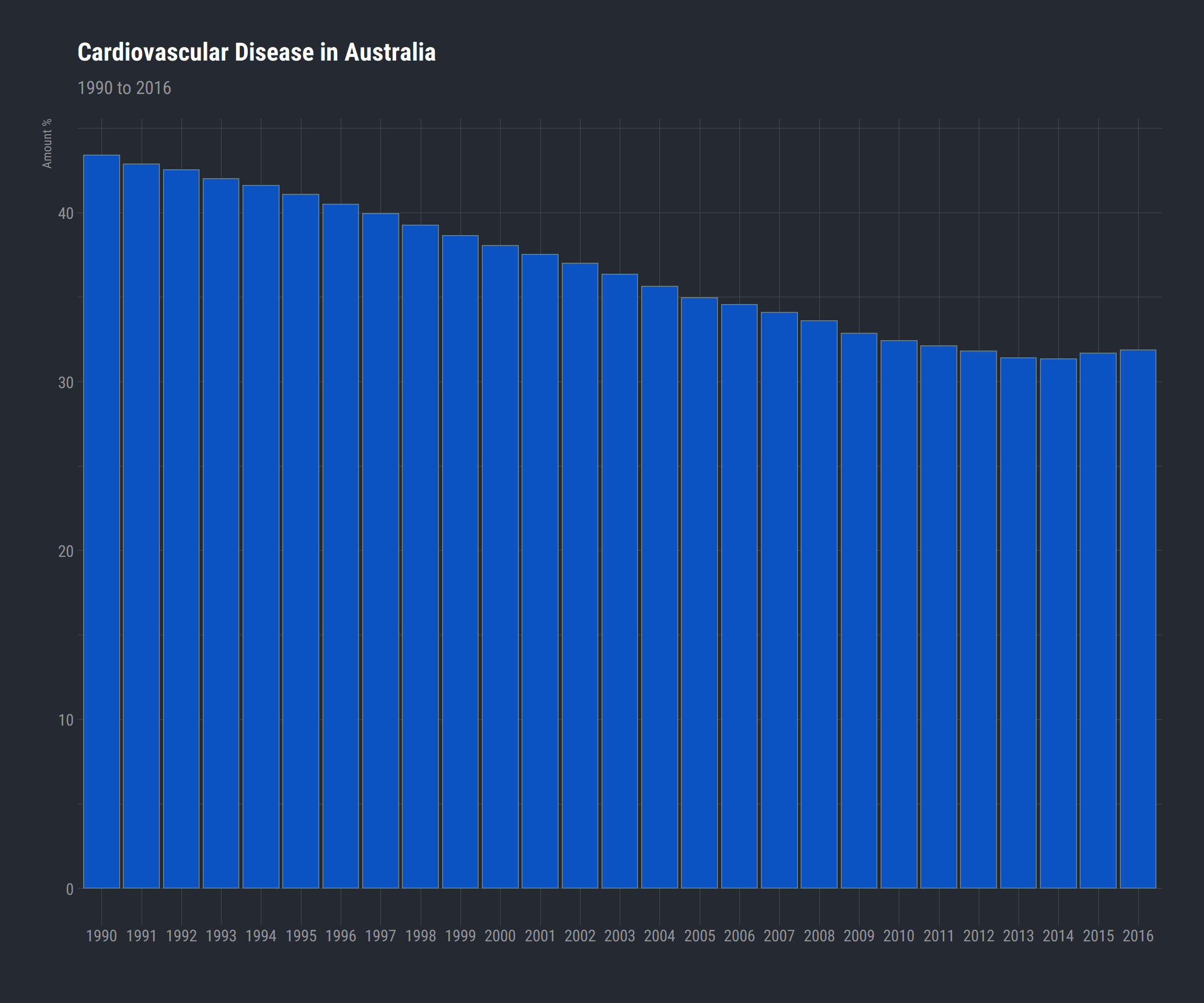
# Drug Related Deaths in Australia
ggplot(Australia) +
  aes(x = year, weight = `Drug disorders (%)`) +
 geom_bar(fill = ft_cols$blue) +
 labs(x = "", y = "Amount %", title = "Drug Related Deaths in Australia", subtitle = "1990 to 2016") +
 theme_ft_rc()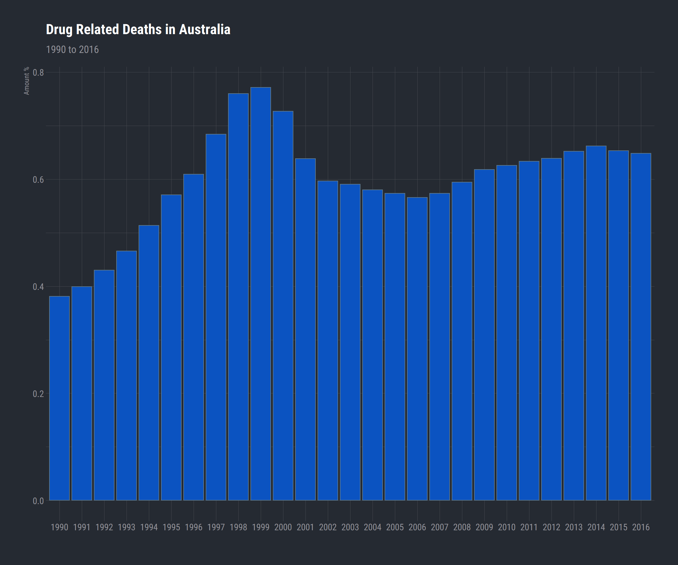
ggplot(Australia) +
  aes(x = year, weight = `Suicide (%)`) +
 geom_bar(fill = ft_cols$blue) +
 labs(x = "", y = "Amount %", title = "Suicides in Australia", subtitle = "1990 to 2016") +
 theme_ft_rc()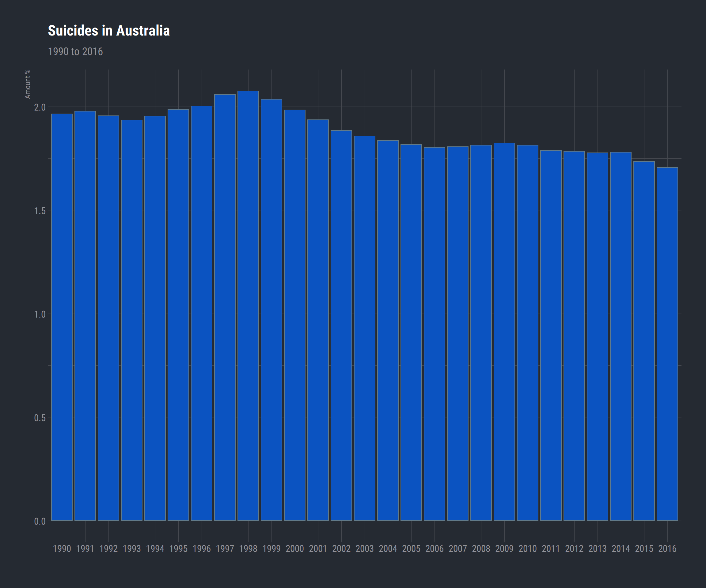
ggplot(Australia) +
  aes(x = year, weight = `Alcohol disorders (%)` ) +
  geom_bar(fill = ft_cols$blue) +
 labs(x = "", y = "Amount %", title = "Alochol Use in Australia", subtitle = "1990 to 2016") +
 theme_ft_rc()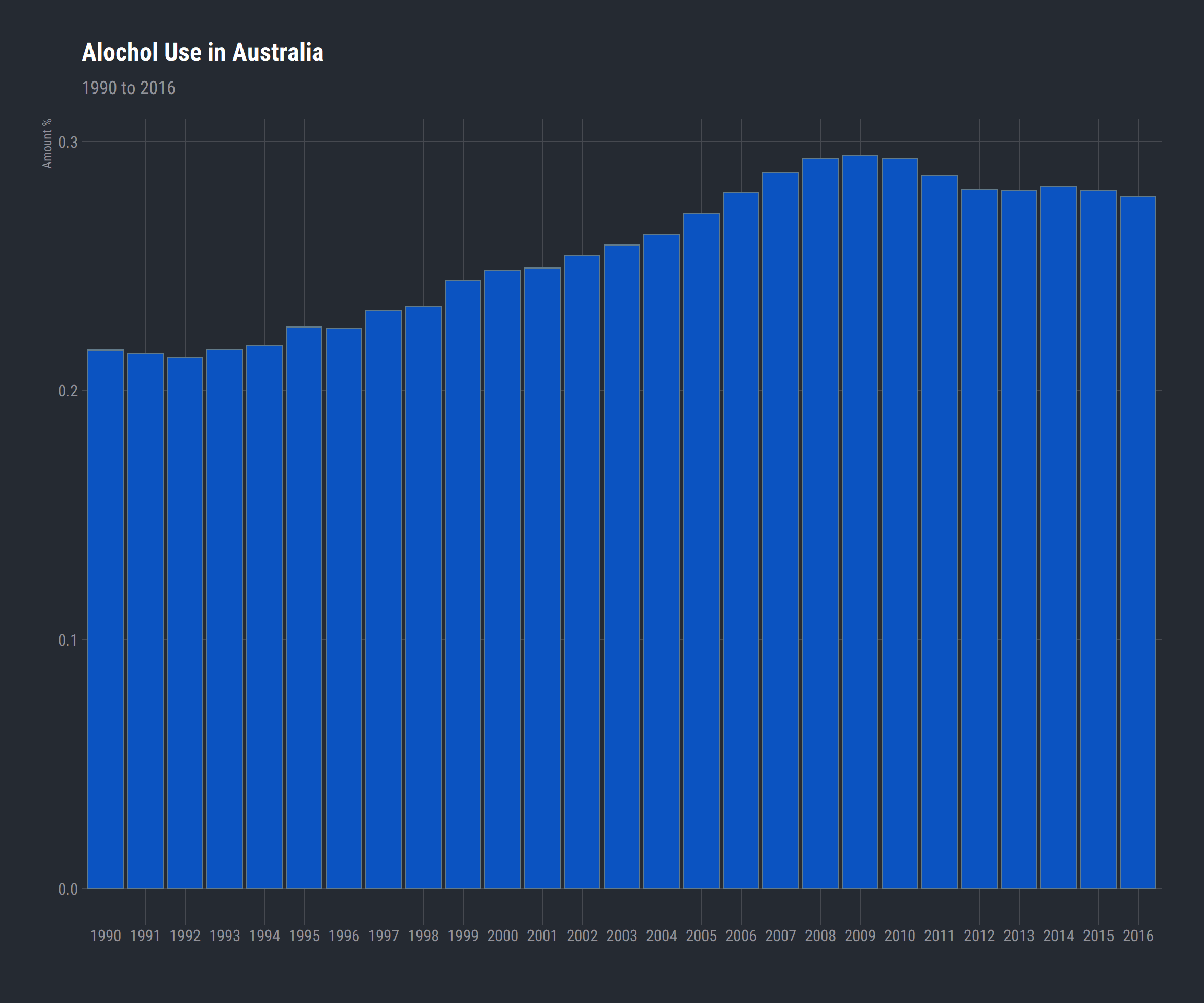
Aaron Willcox
Student
Interests include data wrangling with R and research into neurodevelopmental disorders particularly adult ADHD.